Gradient Descent
In the previous notebook, we looked at simple linear regression and provide a closed-form (analytical) solution for estimating the coefficients/parameters for our model. In this module, let's work on a different parameter estimation technique called Gradient Descent. Gradient descent is a powerful algorithm that is used in a variety of modeling techniques. We explore this technique using the Simple Linear Regression problem
Recall the linear model:
$$ y=\beta_0 + \beta_1*x + \epsilon$$
where:
$y$ is the dependent variable - for example, price of a House
$x$ is the independent variable - for example, sqft of the house
$\epsilon$ is the error
Note that we are trying to estimate $\beta_0$ and $\beta_1$. We do this by defining our cost function and making it our objective to minimize that cost function.
Recall the Cost Function
Our cost function can be mathematically represented as: $$ RSS = \sum_{n=i}^{N} ({y_i - \widehat{y_i}})^2$$
Note that the above formula can be written as: $$ \sum_{n=i}^{N} (y_i - (\widehat{\beta_0} + \widehat{\beta_1}*x))^2 = \sum_{n=i}^{N} (\epsilon_i)^2$$
Conceptual Gradient Descent
In the closed form solution, we derived the parameters each at a time by computing the partial derivative of the cost function for $\beta_0$ and $\beta_1$ individually. In many cases, computers often use matrix methods to compute this estimation.
In fact, the notation for the closed form solution in matrix notation is:
$$ \beta = (H^TH)^{-1}H^Ty$$
where:
$\beta$: vector of all coefficients
$H$: input matrix (matrix of our input variables)
$y$: vector of our predicted variable
Inverting a matrix can be computationally prohibitive, therefore, gradient descent is a much better option. To set up the gradient descent, we need to set up the following dependencies:
- Initialize a vector of our parameters $\beta$. We can initialize parameters to Zero
- Step Size need for parameter approximation. We can set this as a decaying value
- Partial derivative for every parameter we are trying to estimate.
- Updating the parameter:
- Convergence criteria. $$\| \nabla RSS(\beta^{t}) \| > \epsilon$$
The generic partial derivative formular is: $$\frac {\partial RSS(\beta)}{\beta_i} = -2\sum x_i (y_i - \widehat y(\beta))$$
$$\beta_i^{t+1} = \beta_i^{t} - t * \frac {\partial RSS(\beta)}{\beta_i} $$
where:
$t$: stepsize
where:
$\epsilon$: is a predefined torelance
Summarizing the Algorithm
$$while\ \| \nabla RSS(\beta^{t}) \| > \epsilon: $$ $$ for\ i = 0,1,...,D$$
$$\frac {\partial RSS(\beta)}{\beta_i} = -2\sum x_i (y_i - \widehat y(\beta))$$
$$\beta_i^{t+1} = \beta_i^{t} - t * \frac {\partial RSS(\beta)}{\beta_i}$$
Gradient Descent Implementation
Now that we have a summarized version of the algorithm, we can build it from scratch in core python. Below, I demonstrate building a gradient descent class to estimate the parameters $\alpha$ and $\beta$
class SimpleLinearRegression:

    def __init__(self, feature, target):
        self.feature = feature
        self.target = target

    def __str__(self):
        return "Simple Linear Regression Class"

    def gradient_parameter(self, tolerance):
        """ Gradient Descent Algorithm """
        self.alpha = 0
        self.beta = 0
        self.count = 0
        self.stepsize = .001

        error = self.target - (self.alpha + self.beta * self.feature)
        magnitude = abs(np.sum(error))
        while magnitude > tolerance:
            """ Updating the Intercept"""
            self.alpha = self.alpha + self.stepsize*np.sum(error)
            self.beta = self.beta + self.stepsize*np.sum(error*self.feature)

            self.count += 1
            error = self.target - (self.alpha + self.beta * self.feature)
            magnitude = abs(np.sum(error))
        print("Total Updates:", self.count)
        return self.alpha, self.beta
Implementing the Algorithm on Data
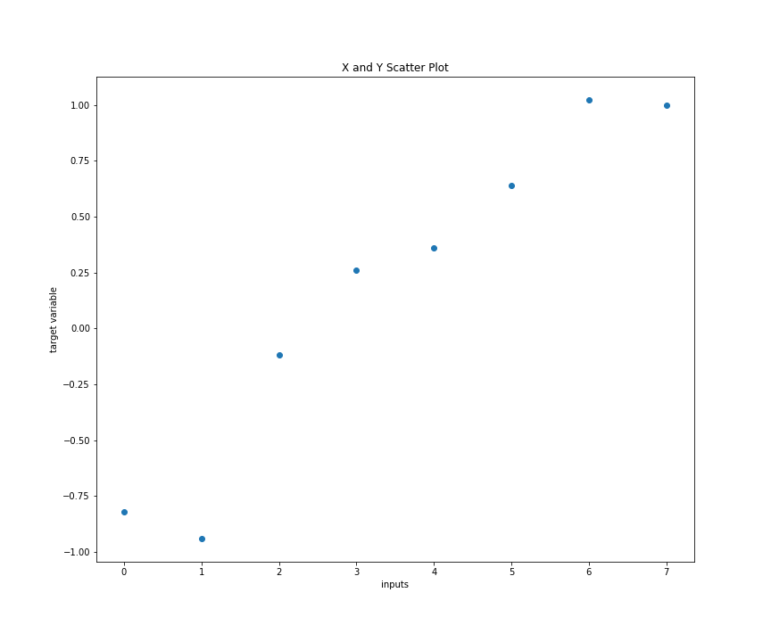
As we did within the Simple Linear Model section, let's estimate the parameters of some linear relationship using this class. Before we do this, we will need to create some raw data with a pre-defined linear relationship. We do this below:
import numpy as np
import pandas as pd
import matplotlib.pyplot as plt
Below we set up some dummy data.
x = np.array([0., 1., 2., 3., 4., 5., 6., 7.])
y = np.array([-.82, -.94, -.12, .26, .36, .64, 1.02, 1.])

plt.figure(figsize=(8,6))
plt.scatter(x, y)
plt.xlabel('inputs'); plt.ylabel('target variable')
plt.title('X and Y Scatter Plot')
With the class already developed and some data generated, we can execute the algorithm and return the estimate.
slr_grad = SimpleLinearRegression(x, y)
alpha, beta = slr_grad.gradient_parameter(0.0001)
alpha, beta We see that the gradient method has iterated over 430 times to update the coefficients. Notice that it is important to set the right tolerance and learning right that will lead to convergence otherwise, gradients can explode to infinity.
Making Predictions
With our parameters estimated, we can now predict and plot our prediction against our data to determine how well we have done.
def prediction(alpha, beta, feature):
    return round( alpha + beta*feature, 3)
preds = prediction(alpha, beta, x)Regression Plot
With our predictions computed, we can now visualize the predictions against the actual observation to see how our model has performed.
plt.figure(figsize=(8,6))
_ = plt.scatter(x, y)
plt.plot(x, preds)
plt.xlabel('inputs'); plt.ylabel('target variable')
plt.title('X and Y Scatter Plot')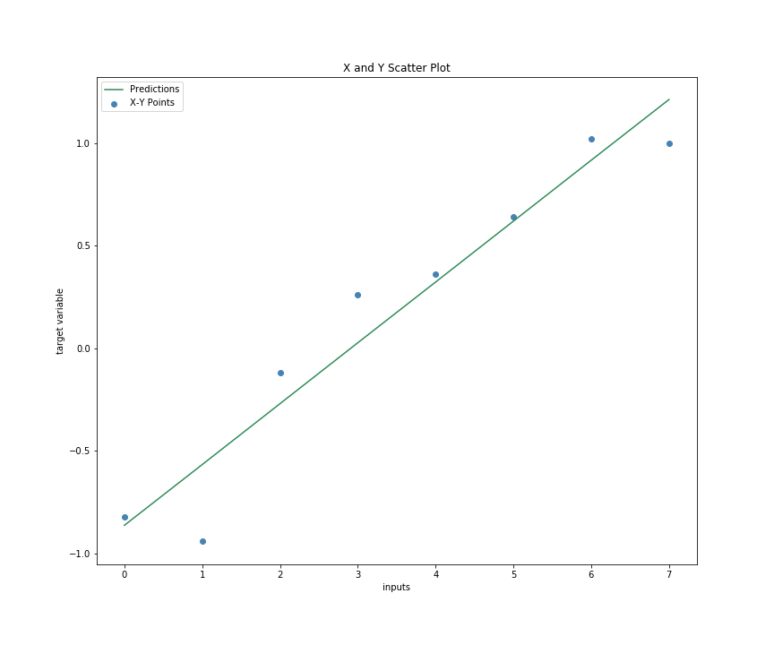
Goodness of Fit: R-Squared
Finally, we can compute the R-squared to contextualize how much variation of target variable y is explained by our model. This also informs us how good our model fits the data
def r_squared(target, prediction):
    ssr = np.sum( (prediction - np.mean(target))**2  )
    sst = np.sum( (target - np.mean(target))**2 )
    return round(100 * ssr/sst , 2)
r_sq = r_squared(y, preds)
r_sq That is a pretty good fit. 93.04% of the variation in the data can be explained in our model. But of course, this is a simple and well-defined problem.
There are a few challenges when implementing the gradient descent method and the biggest one is determining the learning rate. Try this on your date with different learning rates and see what the results turn out. We will cover learning rates in another section.