Logistic Regression
Logistic regression is a statistical method used for binary classification problems, where the outcome variable has two possible categories. Unlike linear regression which predicts continuous values, logistic regression estimates the probability that an observation belongs to a particular class. It uses the logistic function to transform linear combinations of input features into probabilities between 0 and 1, making it particularly useful for predicting outcomes such as yes/no, pass/fail, or default/no default scenarios in financial modeling.
Mathematical Formulation
Logistic regression is used to model the probability of a binary outcome based on one or more predictor variables. We will use the Default dataset from the ISLR package to demonstrate this process.
Recall that the model takes the form:
$$p(y = Default | X) = \beta_0 + \beta_1X$$
With the logistic function, it can be written as:
$$ p(Y) = \frac {e^{\beta_0 + \beta_1 X}} {1 + e^{\beta_0 + \beta_1 X} } $$
The Dataset
For this task, we will use the Default dataset from the ISLR (Introduction to Statistical Learning with R) book. This dataset contains information on whether an individual defaults on their credit card payment along with predictors such as income, balance, and student status. It is an excellent example for practicing logistic regression.
Metadata
default: Indicates whether the individual defaulted on their credit card payment, (Yes, No)
student: Indicates whether the individual is a student. (Yes, No)
balance: The balance on the individual's credit card.
income: The individual's annual income.
Loading the Data
Now lets load the dataset into a data object.
import pandas as pd
import numpy as np
from sklearn.model_selection import train_test_split
from sklearn.linear_model import LogisticRegression
from sklearn.metrics import accuracy_score, classification_report, confusion_matrix, roc_auc_score, roc_curve
import matplotlib.pyplot as plt
import seaborn as sns
# Load the dataset
data = pd.read_csv('datasets/Default.csv')
# Display first few rows to understand structure
print(data.head())
print("\n")
print(data.info())Exploratory Data Analysis (EDA)
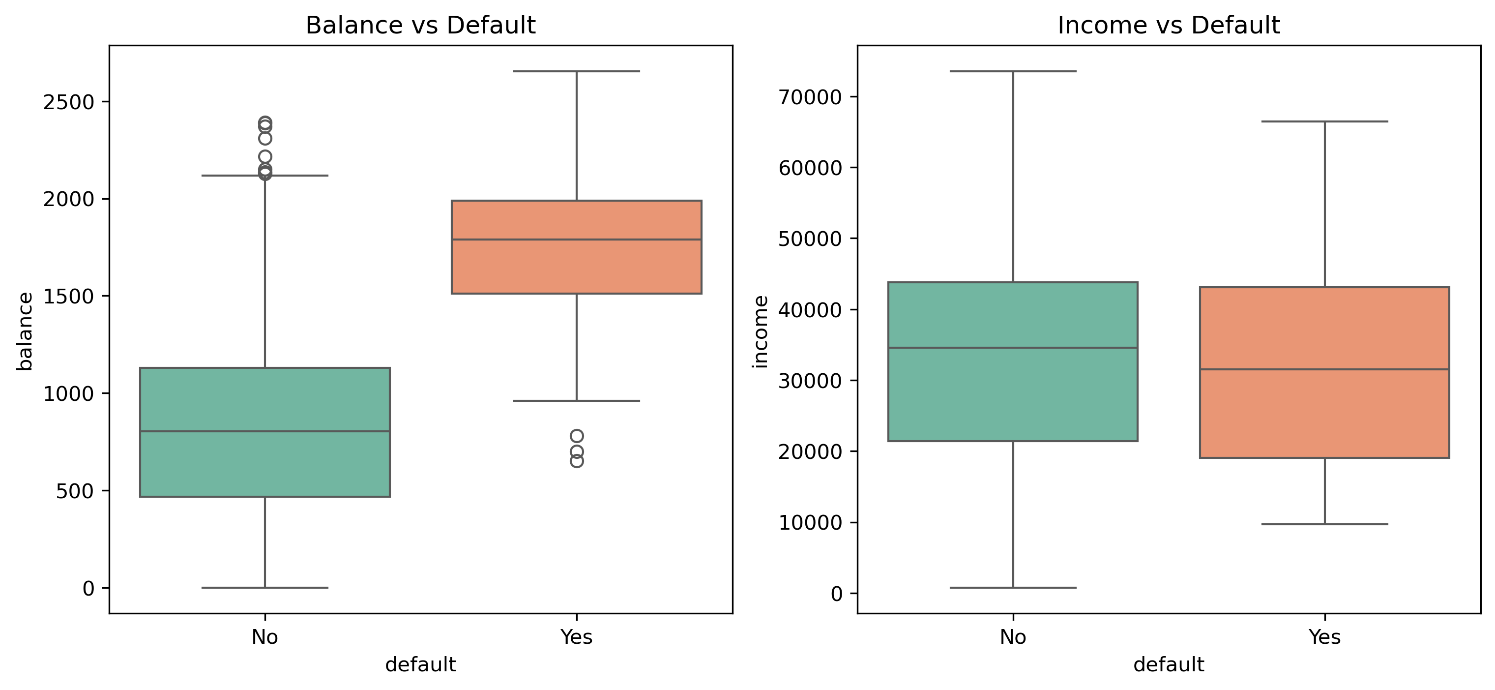
Before modeling, we explore the data to understand distributions and relationships between features and the target variable.
# Visualize relationships between features and default
plt.figure(figsize=(12, 5))
plt.subplot(1, 2, 1)
sns.boxplot(x='default', y='balance', data=data, palette='Set2')
plt.title('Balance vs Default')

plt.subplot(1, 2, 2)
sns.boxplot(x='default', y='income', data=data, palette='Set2')
plt.title('Income vs Default')
plt.show()
# Default count by student status
plt.figure(figsize=(8, 6))
sns.countplot(x='default', hue='student', data=data, palette='viridis')
plt.title('Default Count by Student Status')
plt.show()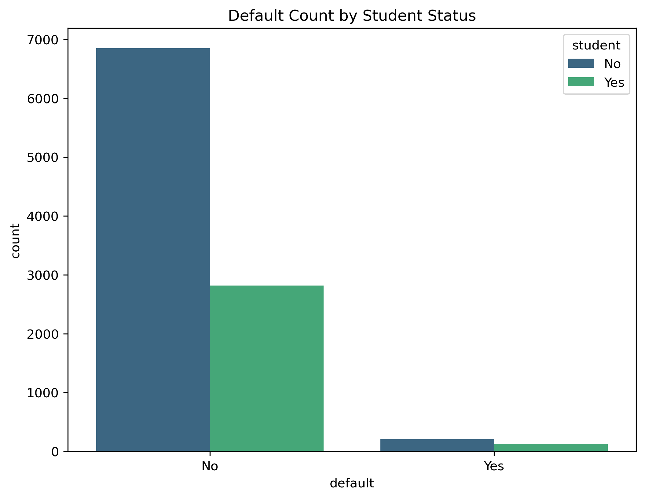
Data Preprocessing
Machine learning models require numerical input. We need to encode the categorical variables 'default' and 'student' into binary format (0 and 1).
# Encoding categorical variables
data['default'] = data['default'].map({'No': 0, 'Yes': 1})
data['student'] = data['student'].map({'No': 0, 'Yes': 1})

# Splitting the data into features (X) and target (y)
X = data.drop('default', axis=1)
y = data['default']

# Splitting into training and testing sets
X_train, X_test, y_train, y_test = train_test_split(X, y, test_size=0.2, random_state=42)
X_train.shape, X_test.shapeModel Training
We will now initialize and train the Logistic Regression model using the training data.
# Initialize the model
model = LogisticRegression()

# Fit the model
model.fit(X_train, y_train)
Model Evaluation
To assess the model's performance, we will look at several metrics including Accuracy, Confusion Matrix, Classification Report, and ROC AUC.
# Predictions
y_pred = model.predict(X_test)
y_prob = model.predict_proba(X_test)[:, 1]

# Metrics
print(f"Accuracy: {accuracy_score(y_test, y_pred)}")
print("\nConfusion Matrix:")
print(confusion_matrix(y_test, y_pred))
print("\nClassification Report:")
print(classification_report(y_test, y_pred))
print(f"\nROC AUC: {roc_auc_score(y_test, y_prob):.4f}")Visualizations
Visualizing the results helps in understanding how well the model is separating the classes.
# Plot Confusion Matrix
plt.figure(figsize=(8, 6))
sns.heatmap(confusion_matrix(y_test, y_pred), annot=True, fmt='d', cmap='Blues',
            xticklabels=['No Default', 'Default'], yticklabels=['No Default', 'Default'])
plt.title('Confusion Matrix - Logistic Regression')
plt.xlabel('Predicted')
plt.ylabel('Actual')
#plt.savefig('logistic_cm.png', dpi=300, bbox_inches='tight')
plt.show()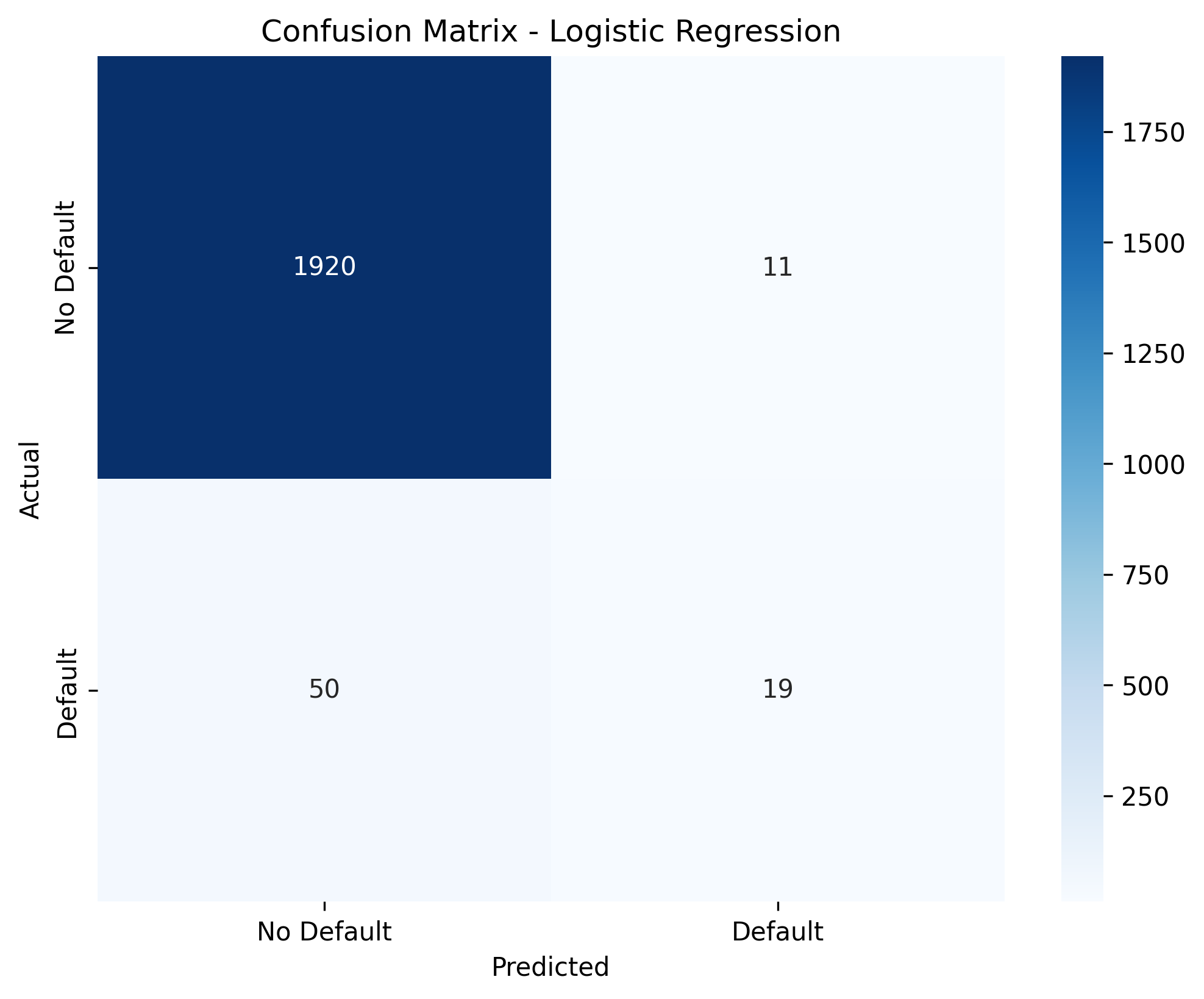
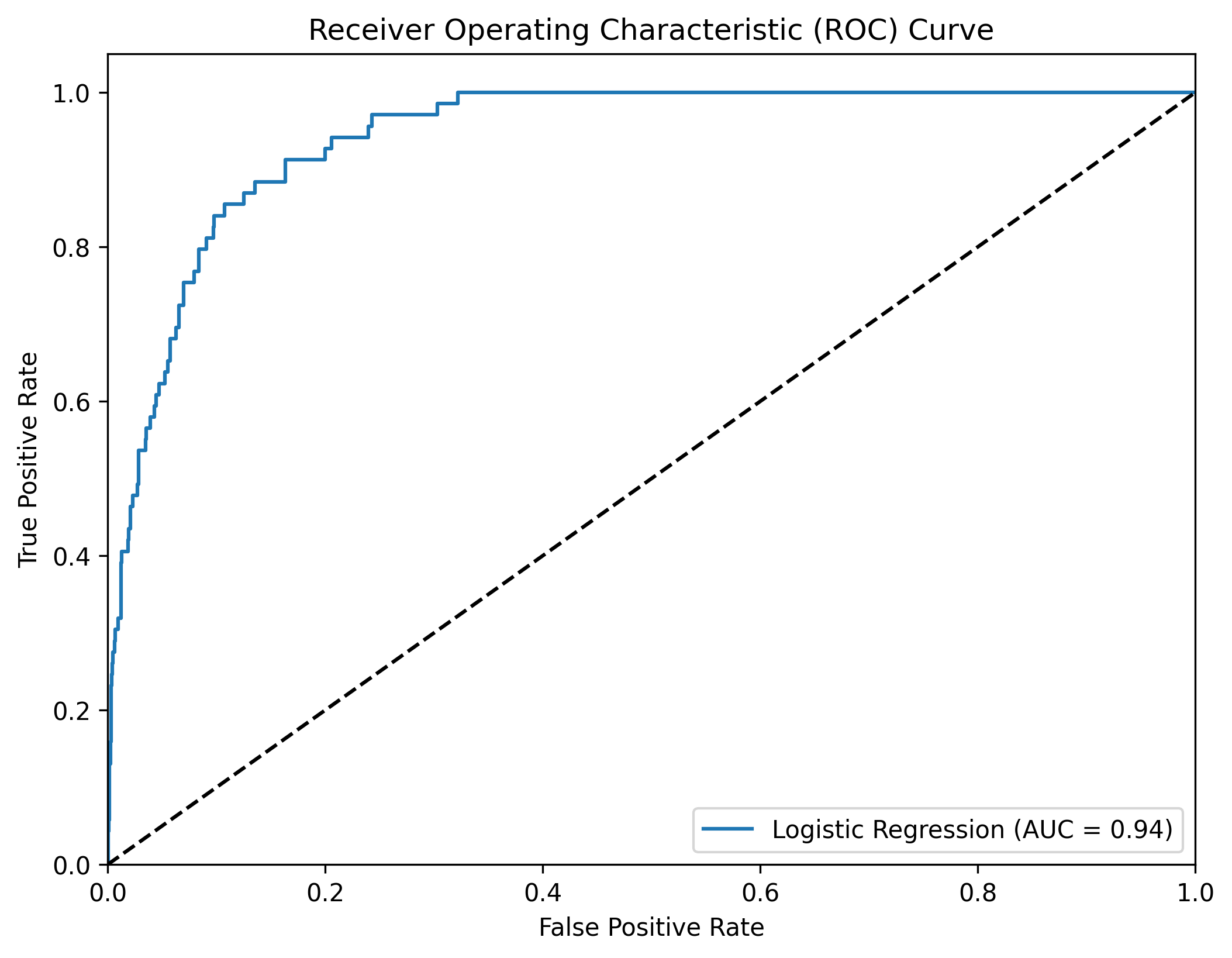
ROC Curve
The ROC curve is a graphical representation of the performance of a binary classifier at various threshold settings. It plots the True Positive Rate (TPR) against the False Positive Rate (FPR) for different threshold values.
# Plot ROC Curve
fpr, tpr, thresholds = roc_curve(y_test, y_prob)
plt.figure(figsize=(8, 6))
plt.plot(fpr, tpr, label=f'Logistic Regression (AUC = {roc_auc_score(y_test, y_prob):.2f})')
plt.plot([0, 1], [0, 1], 'k--')
plt.xlim([0.0, 1.0])
plt.ylim([0.0, 1.05])
plt.xlabel('False Positive Rate')
plt.ylabel('True Positive Rate')
plt.title('Receiver Operating Characteristic (ROC) Curve')
plt.legend(loc="lower right")
#plt.savefig('logistic_roc.png', dpi=300, bbox_inches='tight')
plt.show()