Non-Linear Functions
Non-linear functions are widely used in non-linear regression problems particularly in the business world. A few examples are:
- Estimating the relationship between dollars spend and revenue earned - (diminishing returns)
- Estimate the decaying impact of advertisement over time - (exponential)
In this section, I introduce the most common functions used in non-linear regression particularly focusing on diminishing returns functions and functions' properties. For those working in the business space and seeking to model such relationships as Cost to Revenue, this is a great place to evaluate useful functions to model your data.
Before we begin, let's import the packages we will need to constract the functions and visualize the functional form
import numpy as np
import seaborn as sns
import matplotlib.pyplot as plt

%matplotlib inline
1. Power Function
The power function is commonly used function to model non-linear relationships with a lot of flexibility due to the beta parameter. The formal functional form is:
$$ f(x) = \alpha * x^ \beta $$
where:
$\alpha$: is a scalar parameter for scaling the power function
$\beta$: define the non-linear form with varing values.
In the code below, we see different examples of the power functions in generating both linear relationships i.e. $\beta = 1$ and non-linear relationships i.e. $\beta \neq 1$
def power_function(alpha, beta, x):
    return alpha * x ** beta

x_vals = np.linspace(5, 50, 20 )
pars = list(zip([20 , 20, 20],[ .001, 1, 3]))
y_vals = {'α = {}, β = {}'.format( pars[i][0], pars[i][1]):power_function(pars[i][0],
            pars[i][1],x=x_vals) for i,value in enumerate(pars)}

fig = plt.figure(figsize=(20, 5))
plt.suptitle("Power Functions with Varying β's", y=1.01, fontsize=15)

count = 1
for coeff,y_val in y_vals.items():
    fig.add_subplot( int('13{}'.format(count)))
    sns.lineplot(x=x_vals, y=y_val, label=coeff)
    count += 1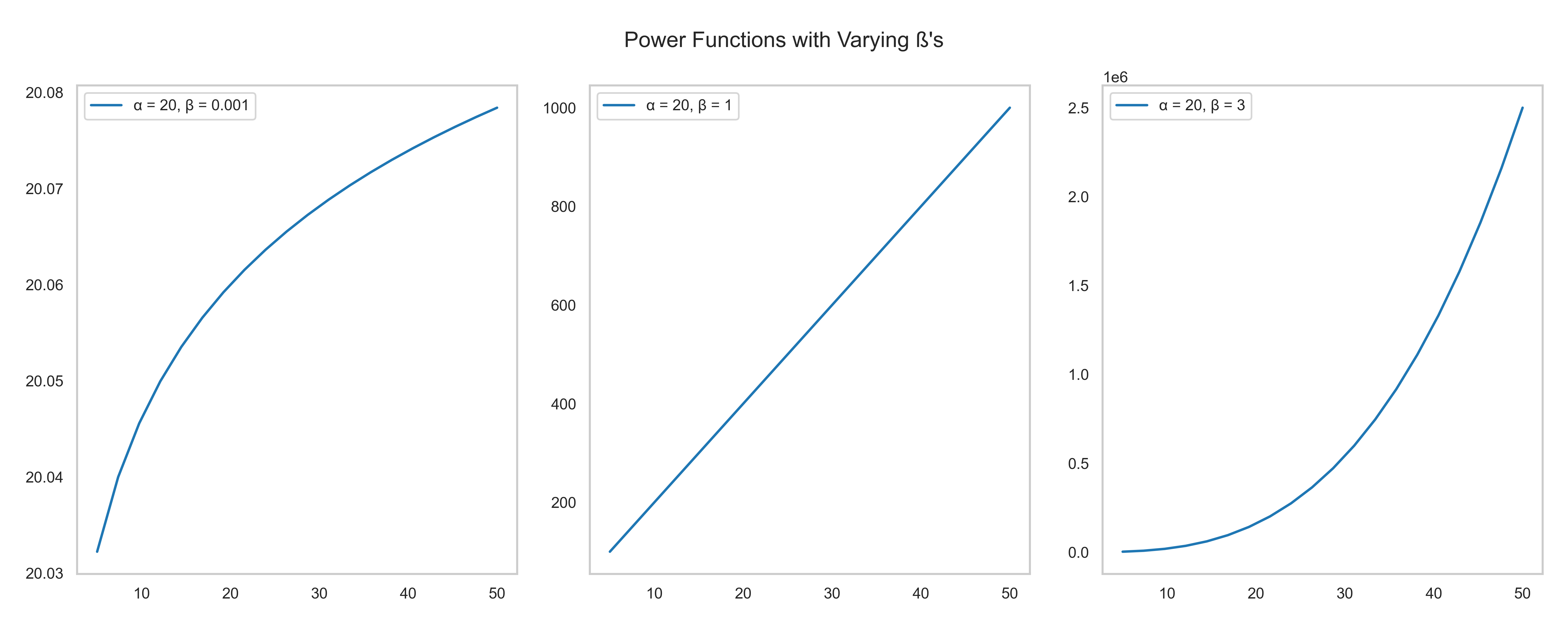
As we see above, by manipulating the $\beta$ parameter, we can use the power function to fit against varying sets of non-linear regression problems. Both diminishing returns, linear and exponential functions can be modeled with the power curve by tuning the beta parameter.
2. Logarithmic Growth Functions
The logarithmic growth model is another mathematical function with good properties that can be used for
modelling diminshing returns. The functional form of the logarithmic growth model is:
$$f(x) = \alpha + \beta * ln(x)$$
where:
$\alpha$: the intercept for the function
$\beta$: tuning parameter for the slope of the growth function
Again with $\alpha$ and $\beta$ parameters, we can control the functional form to return.
Below we see an example of the logarithmic growth functions with varying betas and their response curves.
def log_growth(alpha, beta, x):
    return alpha + beta*np.log(x)

x_vals = np.linspace(1, 50, 20 )
pars = list(zip([20 , 20, 20],[10, 30, 50]))

x_vals = np.linspace(1, 50, 20 )
y_vals = { 'α = {}, β = {}'.format( pars[i][0],
            pars[i][1]):log_growth(pars[i][0], pars[i][1],x=x_vals) for i,value in enumerate(pars)}


fig = plt.figure(figsize=(20, 5))
plt.suptitle("Log Growth Functions with Varying β's", y=1.01, fontsize=15)

count = 1
for coeff,y_val in y_vals.items():
    fig.add_subplot( int('13{}'.format(count)))
    sns.lineplot(x=x_vals, y=y_val, label=coeff)
    count += 1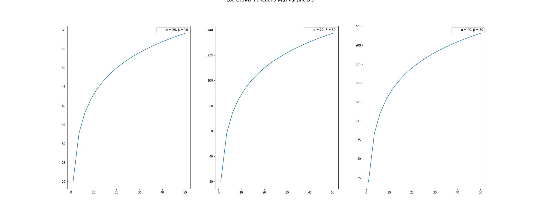
When using the log growth function, remember that the independent variable is scaled to the natural log or base log. This is important in fitting the curve because the outcomes would be scaled by log and may need to be rescaled.
3. Negative Exponetial Functions
Another useful family of functions for non-linear models is the exponetial family which model exponential growth
and decay between two variables. For diminishing returns, we are interested in negative exponetial growth. The
mathematical function of negative exponential growth is:
$$ f(x) = \alpha * (1 − exp^{(−\beta x)})$$
where:
$ \alpha$: tuning parameter for scale
$ \beta $: tuning parameter for exponential trend
For diminishing returns curve, we need $\beta > 0$ must be set as the condition. In the code below, we explore the various conditions. We try the following parameters:
$\alpha = 7$
$\beta = .003$ ~ linear
$\beta = .1$ ~ diminishing returns
$\beta = .2$ ~ strong diminishing returns
def negative_exponential(alpha, beta, x):
    return alpha * (1 - np.exp(-beta * x) )


x_vals = np.linspace(1, 50, 20 )
pars = list(zip([7,7,7],[.003, .1, .5]))

x_vals = np.linspace(1, 50, 20 )
y_vals = { 'α = {}, β = {}'.format( pars[i][0],
            pars[i][1]): negative_exponential( pars[i][0], pars[i][1], x=x_vals) for i,value in enumerate(pars)}


fig = plt.figure(figsize=(20, 5))
plt.suptitle("Negative Exponential Functions with Varying β's", y=1.01, fontsize=15)

count = 1
for coeff,y_val in y_vals.items():
    fig.add_subplot( int('13{}'.format(count)))
    sns.lineplot(x=x_vals, y=y_val, label=coeff)
    count += 1
4. Michaelis-Menten Function
Finally, we look at the Michaelis-Menten function that is finds its root in biology looking at Enzyme reaction.
The functional form can be used for modelling diminishing returns with constrants on parameters. The
mathematical definition of the function is:
$$ f(x) = \frac {\alpha * x} {1 + \beta * x} $$
where:
$\alpha$: scaling parameter for x
$\beta$: tuning parameter for diminishing returns.
To return a diminishing returns form, we need to constrain $\beta \geq 0$. In the example below, we see variations of these functions based on different $\beta$ values. We visualize the following values:
$\alpha = 7$
$\beta = .01$ ~ linear to dim returns
$\beta = .05$ ~ diminishing returns
$\beta = .1$ ~ diminishing returns
$\beta = 1$ ~ strong diminishing returns
def michaelis_menten(alpha, beta, x):
    return (alpha*x)/(1 + beta*x)

pars = list(zip([7,7,7,7],[.01, .05, .1, 1]))

x_vals = np.linspace(1, 50, 20 )
y_vals = { 'α = {}, β = {}'.format( pars[i][0],
            pars[i][1]):michaelis_menten(pars[i][0],pars[i][1],x=x_vals) for i,value in enumerate(pars)}


fig = plt.figure(figsize=(20, 4))
plt.suptitle("Michaelis-Menten Functions with Varying β's", y=1.01, fontsize=15)

count = 1
for coeff,y_val in y_vals.items():
    fig.add_subplot( int('14{}'.format(count)))
    sns.lineplot(x=x_vals, y=y_val, label=coeff)
    count += 1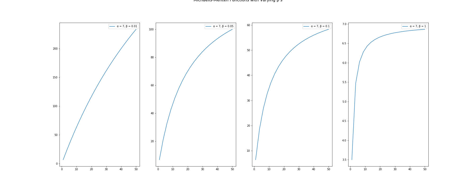
The functional forms above are useful particularly in business to model non-linear relationships such as diminishing returns and growth models. In the next section, we fit diminishing returns curve on some fictitious marketing data to implement general non-linear regression techniques.