Non-Linear Regression

In those notebook, we explore fitting a non-linear regression model on data that is not linearly related. The objective to demonstrate the implementation of non-linear regression and in this particular case, diminishing returns relationship between two variables.

We begin by importing all the packages that we are going to use.

import numpy as np
import pandas as pd
import seaborn as sns
import matplotlib.pyplot as plt
from scipy.optimize import curve_fit

%matplotlib inline

The data we are using in this example is purposely generated with a strong diminishing returns trend to demonstrate non-linear regression.

dim_data = pd.read_csv('data.csv')
dim_data.head()

	x-vals	y-vals
0	18.344701	5.072228
1	79.865377	7.158815
2	85.097875	7.262765
3	10.521103	4.254581
4	44.455587	6.281867

Visualizing the Data

With our data in a dataframe, let's visualize the x and y values in a scatter plot and determine whethere there exists a non-linear relationship between the two variables.

plt.figure(figsize=(8,6))
sns.scatterplot(data=dim_data, x='x-vals', y='y-vals')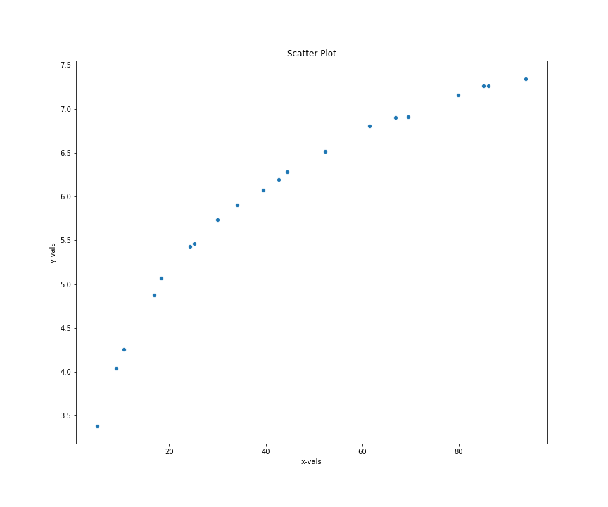

The trend clears shows a dimishing returns relationship between x and y values. To model this relations, we can select from one of the many non-linear fuctions available in the non-linear regression function notes. Some good options are:

1. Log Growth Functions
2. Power Functions

Diminishing Returns Function

We will use both the log-growth and power functions to build our diminishing returns model and compare the fit against each other. To do this, we need to define the both functions and fit the functions using curve_fit method available with scipy. Note that it is imported above.

def log_growth(x, alpha, beta ):
    return alpha + beta*np.log(x)

def power_function(x, alpha, beta):
    return alpha * x ** beta

When defining the functions above, it's important to make sure that the x input comes first in the function. Otherwise, your fits may not work at all.

Fitting the Functions in Regression

With the functions already defined, we fit the function to the curve_fit model by passing the functions and our data.

log_params = curve_fit(log_growth, dim_data['x-vals'].values, dim_data['y-vals'].values)[0]
power_params = curve_fit(power_function, dim_data['x-vals'].values, dim_data['y-vals'].values)[0]
    
log_params, power_params

(array([0.97977689, 1.40156915]), array([2.39574961, 0.25116701]))

Our curve has been fit and our parameters for both functions are estimated. We observe that the beta parameters are more comparable with the alpha parameters varying. Log function has a higher alpha coefficient than the log growth.

Making Predictions

With out paramater in hand, we can make the predictions and plot the predictions to see the fit on both function. In the code below, we predict the values with both functions and plot the predictions against the actual observations.

x_vals = np.linspace( dim_data['x-vals'].min(), dim_data['x-vals'].max(), 20 )
log_pred = log_growth(alpha= log_params[0], beta= log_params[1], x=x_vals)
pwr_pred = power_function(alpha= power_params[0], beta= power_params[1], x=x_vals)


plt.figure(figsize=(8,6))
sns.scatterplot(data=dim_data, x='x-vals', y='y-vals', label='Actual Data')
sns.lineplot(x=x_vals, y=log_pred, label='Log Growth Fit')
sns.lineplot(x=x_vals, y=pwr_pred, label='Power Function Fit')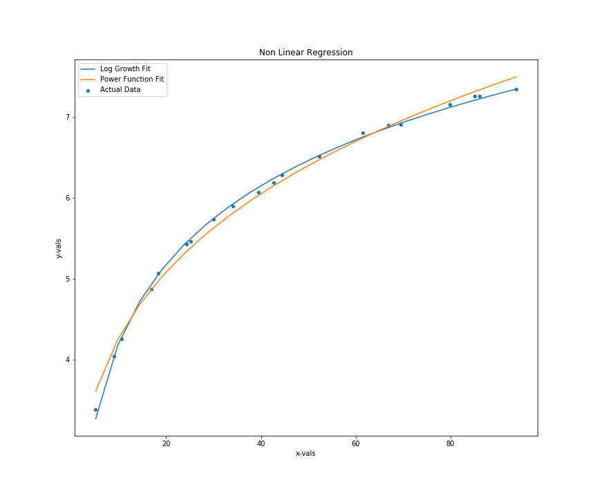

Fit Measurement using R-Squared

We can see from the fit above that both function do a pretty good job at fitting the diminishing returns. However, we can assess their respective performance with an objective metric - R-Squared. $R^2$

As we have seen before, R-Squared measures how well our model explains the variation on y based on changes in x. We create a function and compute the R-Squared below.

def r_squared( actual , prediction):
    ssr = np.sum( (prediction - np.mean(actual))**2 )
    sst = np.sum( (actual - np.mean(actual))**2  )
    return round(100 * ssr/sst, 3)

power_rsquared = r_squared(dim_data['y-vals'], pwr_pred)
log_rsquared = r_squared(dim_data['y-vals'], log_pred)

power_rsquared, log_rsquared

(94.225, 95.22)

Note:

It is important to understand the nature of the functions we are using because power functions only hit flattened curve with x input approaching $\infty$. Obviously this is extrapolation because we have not observations at higher levels of x to determine what the case would be. In that case, I'd probably use the log-growth curve as my selected model.