Linear Regression
Linear regression is a classical and perhaps the most widely used machine learning technique to estimate/predict the outcome of a target metric based on other variables. In the case of simple linear regression, our goal is to estimate the target metric based on another variable. For example, we can estimate the price of a house based on the square-feet of the house. The linear regression model takes the form below:
Equation Form
$$ y=\beta_0 + \beta_1*x + \epsilon$$
where:
$y$ is the dependent variable - for example, price of a House
$x$ is the independent variable - for example, sqft of the house
$\epsilon$ is the error
Based on the equation above, we want to estimate the parameters $\beta_0$ and $\beta_1$, such that with an input $x$, we can predict the resulting $y$ value. You can think of randomly assigning values to $\beta_0$ and $\beta_1$ but we will not be able to determine which values provide the closest correct value of $y$. This is where the measure of fit comes into play.
Before we go any further let's generate some data with a linear relationship.
import numpy as np
import pandas as pd
import matplotlib.pyplot as plt

%matplotlib inline
Let's create some data that have some linear relationship and generate a dataframe with these values
x = np.array([0., 1., 2., 3., 4., 5., 6., 7.])
y = np.array([-.82, -.94, -.12, .26, .36, .64, 1.02, 1.])

data = pd.DataFrame(list(zip(x,y)), columns=['x', 'y'])
data.head()| x | y | |
|---|---|---|
| 0 | 0.0 | -0.82 |
| 1 | 1.0 | -0.94 |
| 2 | 2.0 | -0.12 |
| 3 | 3.0 | 0.26 |
| 4 | 4.0 | 0.36 |
Visualizing the data
We can visualize the random data we generated above to determine if a linear model is appropriate.
plt.figure(figsize=(8,6))
plt.scatter(data.x, data.y)
plt.xlabel('inputs'); plt.ylabel('target variable')
plt.title('X and Y Scatter Plot')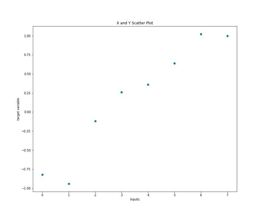
Based on the visual above we see that there is a general linear relationship between x and y that can be expressed in our equation form.
Measure of Fit
Measure of fit defined how good our parameters are at making predictions. We can simply look at the overall difference between predicted values of all observations against the actual values to determine the overall measure of fit. We can do this by computing the residual:
$$residual = y - \widehat{y}$$ where:
$y: actual\ value\ of\ observations$
$\widehat{y}: predicted\ value\ of\ observations$
To obtain the overall difference, we can take the sum of residuals, however, we lose information about the measure of fit given that some values will be over-predicted and some under-predicted. To reconcile this, we compute the sum of squared residuals.
Mathematically:
$$ RSS = \sum_{n=i}^{N} ({y_i - \widehat{y_i}})^2$$
Note that the above formula can be written as: $$ \sum_{n=i}^{N} (y_i - (\widehat{\beta_0} +
\widehat{\beta_1}*x))^2 = \sum_{n=i}^{N} (\epsilon_i)^2$$
Estimating the Parameters
Now that we have a measure of fit, we need to find the values of $\beta_0$ and $\beta_1$ that minimized the measure of fit. That is find the values of $\beta_0$ and $\beta_1$ that provide the lowest sum of squared error (RSS). Our cost function is RSS and we then write our objective function as (minizing the cost function):
$$\min_{\beta_0, \beta_1} \sum_{n=i}^{N} (y_i - (\widehat{\beta_0} + \widehat{\beta_1}*x))^2$$
Luckily, the cost function is a convex function, therefore we can use gradients to solve for $\beta_0$ and $\beta_1$ that minimize the cost function. Below is the solutions:
Closed-Form Solution
We explore the analytical solutions to determining our parameters case by case for the individual parameters
Case 1: $\beta_0$
$$ \frac{\partial RSS(\beta_0, \beta_1)} {\partial \beta_0} = \sum 2[y_i - (\widehat{\beta_0} + \widehat{\beta_1} x_i)](-1) $$
Equate the partial to Zero:
$$ 0 = -2 \sum y_i -\sum \widehat{\beta_0} - \sum \widehat{\beta_1} x_1 $$ $$\sum \widehat{\beta_0} = \sum y_i - \widehat{\beta_1} \sum x_i$$
Recall, the sum of a constant is equal to constant multiplied by n:
$$n\widehat{\beta_0} = \sum y_i - \widehat{\beta_1} \sum x_i$$ $$\widehat{\beta_0} = \frac {\sum y_i}{n} - \frac{ \widehat{\beta_1} \sum x_i} {n}$$
Therefore: $$\widehat{\beta_0} = \bar y - \widehat{\beta_1}*\bar x $$
Case 2: $\beta_1$
$$ \frac{\partial RSS(\beta_0, \beta_1)} {\partial \beta_0} = \sum 2[y_i - (\widehat{\beta_0} + \widehat{\beta_1} x_i)](-x_i)$$ Equate the partial to Zero: $$ 0 = -2 \sum y_i x_i - \sum \widehat{\beta_0} x_i - \sum \widehat{\beta_1} x_1^2 $$ $$ 0 = -2 \sum y_i x_i - \widehat{\beta_0} \sum x_i - \widehat{\beta_1} \sum x_1^2 $$ Substitute $\beta_0$ in the equation: $$ 0 = -2 \sum y_i x_i - (\bar y + \widehat{\beta_1} \bar x) \sum x_i - \widehat{\beta_1} \sum x_1^2 $$ $$ 0 = \sum y_i x_i - \bar y \sum x_i + \widehat{\beta_1} \bar x \sum x_i - \widehat{\beta_1} \sum x_1^2 $$ We can simplify the equation using summation rules to: $$ \widehat {\beta_1} = \frac {\sum x_i y_i - n\bar x^2} {\sum x_i^2 - n\bar x^2} $$ $$ \widehat {\beta_1} = \frac {\sum (x - \bar x) (y - \bar y)} {\sum (x - \bar x)^2} = \frac {Cov(X,Y)}{Var(x)}$$
Python Implementation
Now that we have the theory broken down, let's implement this closed solution using python. Below we build a python class that has computes the value of parameters that minimize the cost function.
class SimpleLinearRegression:

    def __init__(self, feature, target):
        self.feature = feature
        self.target = target

    def __str__(self):
        return "Simple Linear Regression Class"

    def closed_form_solution(self):
        numerator = np.sum((self.feature - np.mean(self.feature)) * (self.target - np.mean(self.target)))
        denominator = np.sum((self.feature - np.mean(self.feature))**2)
        beta = numerator/denominator
        alpha = np.mean(self.target) - beta*(np.mean(self.feature))
        return alpha, beta

    def residual_sum_squares(self, alpha, beta):
        return np.sum((self.target - (alpha + beta*self.feature))**2)

    def prediction(self, alpha, beta):
        return alpha + beta*self.feature
Now let's run the regression model
slr_model = SimpleLinearRegression(data.x, data.y)

alpha, beta = slr_model.closed_form_solution()

print('Alpha is {} ,'.format( round(alpha, 2) ),'Beta is {}'.format( round(beta, 2)))
print('RSS is', round( slr_model.residual_sum_squares(alpha, beta), 2))Regression Plot
Because we have calculated the parameters, we can now predict the values of our data and plot the predictions again the original dataset to determine how well we have done.
data.pred = slr_model.prediction(alpha=alpha, beta=beta)

plt.figure(figsize=(8,6))
_ = plt.scatter(data.x, data.y)
plt.plot(data.x, data.pred)
plt.xlabel('inputs'); plt.ylabel('target variable')
plt.title('X and Y Scatter Plot')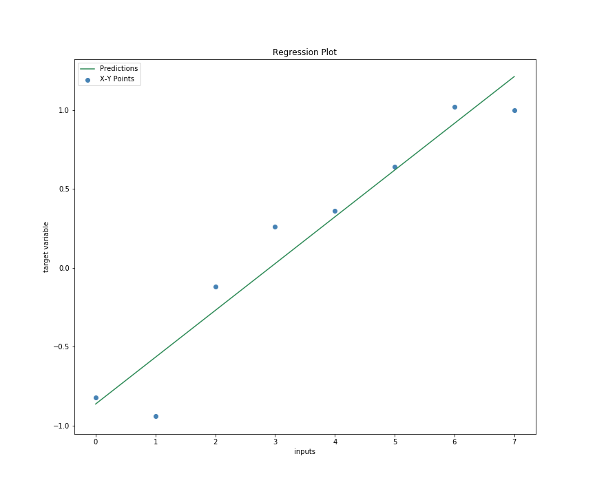
We can see that our model fits the data quite decently. However, to understand how well our model is performing, we need to use a metric that tells how well our models fit.
R-Squared
By definition, r-squared is the amount of variation of y that is explained by our model. To compute the R-Squared, we use the following formular: $$ r^2 = \frac {SSR} {SST}$$
where:
SSR = Sum of Squares Residual
SST = Sum of Square Total Error
In python, we use the following function.
def r_squared( target, prediction):
    ssr = np.sum( (prediction - np.mean(target))**2 )
    sst = np.sum( (target - np.mean(target))**2  )
    return round(100 * ssr/sst, 3)
r_sq = r_squared(data.y, data.pred)
r_sqOur r-squared is at 93% which say that 93% of the variable of target variable y is explained by the variation of x. This is a good result.
Implementation with Sklearn
We can implement the above solution with sklearn which has powerful solvers with fairly minimal code
from sklearn import linear_model

model = linear_model.LinearRegression(fit_intercept=True)
model.fit(data[['x']], data['y'])Model Coefficients
Now we can look at returning the model coefficients from sklearn. Notice the result is equivalent to our closed form solution.
round( model.coef_[0], 3), round( model.intercept_, 3)Notice the resulting coefficients match the closed solution and therefore we expect to get the same prediction.
This concludes the introduction to linear regression. In the next section, we will deal with using gradient descent for parameter estimation.