Beta Distribution
The beta distribution is one of the most important distributions in Bayesian statistics particularly because of its usefulness as a prior for random variables whose domain is between $0$ and $1$. Such random variables like the click-through rate or conversion rate are binomially distributed random variables whose proportional outcome is a continuous variable.
The beta distribution takes two parameters $\alpha$ and $\beta$. The two parameters can often represent the success and failure counts which makes the distribution useful as a prior distribution for binomial and Bernoulli experiments in bayesian statistics.
We can mathematically represent the beta distribution as:
$$ X \sim Beta( \alpha, \beta ) $$
where:
$X$: random variable X and $ 0< x < 1 $
$\alpha$: positive real values
$\beta$: positive real values
Beta Random Variable
The beta method on scipy's can be used to create a random variable by specifying the parameters $\alpha$ and $\beta$, and providing the scale of the random variable within the interval $0$ and $1$.
The function arguments are:
$a$ = $\alpha$ parameter
$b$ = $\beta$ parameter
$loc$ = lower bound $x$
$scale$ = upper bound $x$
from scipy.stats import beta
import matplotlib.pyplot as plt

sim_beta = beta.rvs( a=1, b=1, loc=0, scale=1 ,size=30 )
sim_betaNotice that the random observations in the beta distribution are all contained in the domain specified between the $loc$ and $scale$ values.
Visualization Beta Random Variable
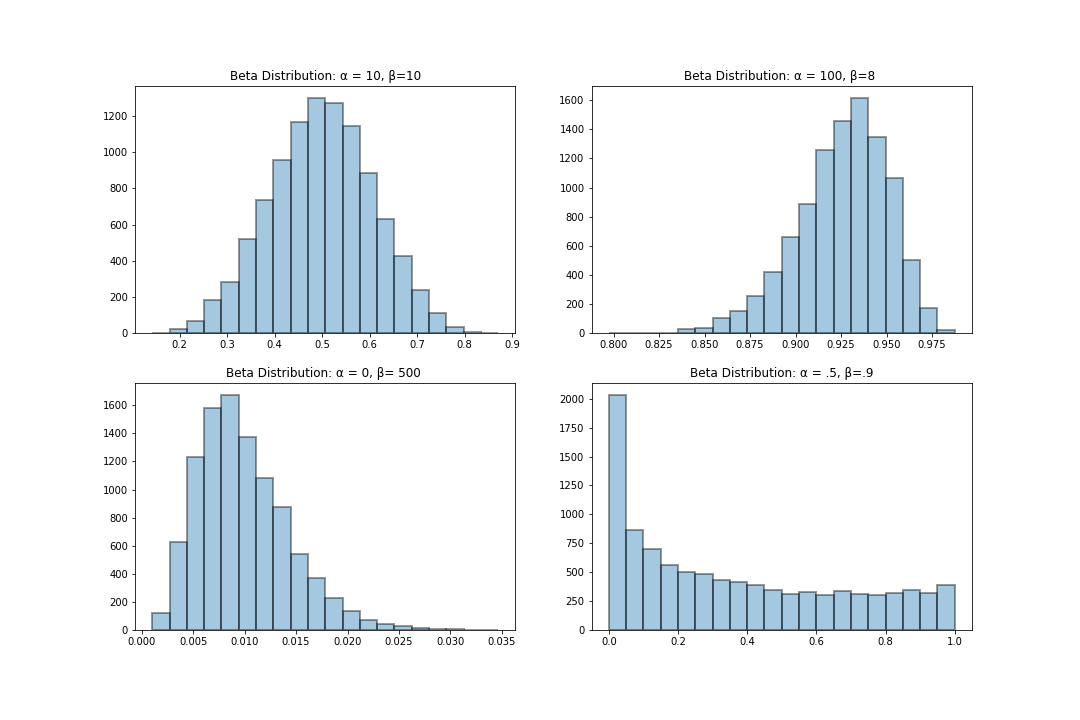
Below, I provide a visualization of the bar plots for beta random variables with varying $\alpha$ and $\beta$ parameters. Notice how the shape of the distributions changes with changes in the parameters. Notice that the changes in the distribution shape is influenced by the magnitude of the $\alpha$ and $\beta$ parameters. That is:
import seaborn as sns
import matplotlib.pyplot as plt

%matplotlib inline
%config InlineBackend.figure_format = 'retina'

fig = plt.figure(figsize=(15,10))

fig.add_subplot(221)
sim_beta = beta.rvs( a=10, b=10, loc=0, scale=1 ,size=10000 )
sns.distplot( sim_beta, kde= False, bins=20, hist_kws=dict(edgecolor="k", linewidth=2) )
plt.title('Beta Distribution: α = 10, β=10')

fig.add_subplot(222)
sim_beta = beta.rvs( a=100, b=8, loc=0, scale=1 ,size=10000 )
sns.distplot( sim_beta, kde= False, bins=20, hist_kws=dict(edgecolor="k", linewidth=2) )
plt.title('Beta Distribution: α = 100, β=8 ')

fig.add_subplot(223)
sim_beta = beta.rvs( a=5, b=500, loc=0, scale=1 ,size=10000 )
sns.distplot( sim_beta, kde= False, bins=20, hist_kws=dict(edgecolor="k", linewidth=2) )
plt.title('Beta Distribution: α = 0, β= 500 ')

fig.add_subplot(224)
sim_beta = beta.rvs( a=.5, b=.9, loc=0, scale=1 ,size=10000 )
sns.distplot( sim_beta, kde= False, bins=20, hist_kws=dict(edgecolor="k", linewidth=2) )
plt.title('Beta Distribution: α = .5, β=.9')
Probability Density Function
The probability density function of the beta distribution is defines as follows:
$$ p(x) = \begin{cases} \frac { x^{\alpha - 1}(1 - x)^{\beta - 1}} {B(\alpha, \beta)} & \text{ for } 0< x < 1 \\ 0 & \text{ for } x < 0\ or\ x\ > 1 \end{cases} $$
$$ B( \alpha, \beta ) = \frac { \Gamma (\alpha) \Gamma (\beta)} {\Gamma (\alpha + \beta) } = \frac { (\alpha -1 )! (\beta - 1)!} { (\alpha + \beta -1)!} $$
where:
$\alpha:$ positive real number parameter
$\beta:$ positive real number parameter
$B(\alpha, \beta):$ is the beta function with parameters $\alpha$ and $\beta$
Example:
Suppose that a landing page generally follows a beta distribution with $\alpha = 46$ and $\beta = 21$. What is the probability that the conversion rate over a random sample is at least 20% points higher than the mean?
For this question, we first need to compute the mean of the distribution and determine the exact value that is 20% higher of the mean.
mean = 46/(46 + 21)
1 - beta.cdf(x= mean+.2, a=46, b=21, loc=0, scale=1 )Expected Value
The expected value of the beta distribution is approximated by:
$$ E(X) = \frac {\alpha}{\alpha + \beta} $$
Example:
Compute the mean of a beta distribution with $\alpha = 20$ and $\beta = 21$. Notice that the values converge
with a higher sampling size.
random_v = beta.rvs( a=20, b=21, loc=0, scale=1, size=100000 )
random_v.mean(), 20/(20 + 21)Variance
The variance of the beta distribution is approximated by:
$$ Var(X) = \frac {\alpha \beta}{(\alpha + \beta + 1)( \alpha + \beta )^2 } $$
Example:
Compute the variance of a beta distribution with $\alpha = 20$ and $\beta = 21$. Notice that the values converge
with a higher sampling size.
random_v = beta.rvs( a=20, b=21, loc=0, scale=1, size=100000 )
random_v.var(), (20 * 21 )/((20 + 21 + 1)*( 20 + 21)**2)Standard Deviation
The standard deviation is approximated by the formular:
$$ std(x) = \sqrt{\frac {\alpha \beta}{(\alpha + \beta + 1)( \alpha + \beta )^2 } } $$
Example:
Compute the standard deviation of a beta distribution with $\alpha = 20$ and $\beta = 21$. Notice that the
values converge with a higher sampling size.
import numpy as np
random_v = beta.rvs( a=20, b=21, loc=0, scale=1, size=100000 )
random_v.std(), np.sqrt( (20 * 21 )/((20 + 21 + 1)*( 20 + 21)**2) )