Binomial Distribution

The binomail distribution models the probability of a random variable with binary sample space when an experiment is repeated n-times. For example, what is the probability of getting an even number when a dice is rolled $10$ times.

Mathematically: $$ X \sim \beta_{p, n} $$ where:
$X$: is a random variable
$p$: probability of success
$n$: number of trials

Binomial Random Variables

As seen above, the binomial distribution takes two paraters $p$ and $n$. We can generate a binomial random variable by providing the binomial class the $p$ and $n$ parameters. Notice that generating a binomial random variable will return the total number of successes from a binomial distribution with $p$ probability and $n$ trials

from scipy.stats import binom
import matplotlib.pyplot as plt

x_binom = binom.rvs(p=.5, n=10, size=100)
x_binom

array( [4, 7, 3, 3, 6, 2, 4, 5, 4, 4, 5, 7, 6, 3, 6, 3, 7, 4, 7, 4, 6, 8, 5, 3, 6, 4, 3, 9, 6, 5, 8, 7, 4, 4, 6, 6, 5, 6, 5, 6, 5, 6, 3, 5, 5, 7, 6, 7, 3, 4, 3, 4, 5, 4, 4, 6, 3, 4, 6, 4, 8, 6, 7, 5, 8, 5, 4, 5, 2, 4, 3, 6, 7, 7, 7, 7, 6, 1, 5, 5, 2, 3, 2, 5, 6, 3, 8, 3, 4, 5, 7, 7, 4, 5, 3, 3, 4, 7, 4, 5])

Visualize the distribution plot

We can visualize the counts of successes based on the $n$ trials with $p$ probability of success over a sample of 10000. Notice that the binomial distribution converges to the expected value $5$.

x_binom = binom.rvs(p=.5, n=10, size=10000)

fig = plt.figure(figsize=(8,5))
_ = plt.hist(x_binom, bins=100)
plt.xlabel('Binomial Success')
plt.ylabel('Frequency')
plt.title('Binomial Distribution of Success')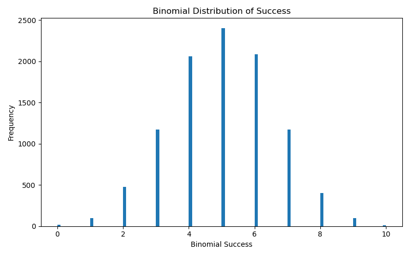

Probability Mass Function

The probability mass function is mathematically defined as:

$$ P(x) = \binom{n}{k}(p^k)(1-p)^{n-k} $$

where:
$n$: is the number of trials
$k$: is the number of success
$p$: is the probability of success

The above equation is the pmf given n-trials and n-success. To motivate the use of the probability mass function, let's use an example problem below.

Example Problem:
What is the probability of getting 4 out of 6 questions correct with each question having 4 multiple choices.

From this example, we have the following information:
n = 6
k = 4
p = .25

We can calculate this is in python pretty easily using the pmf function

from scipy.special import comb

prob_4 = comb(6, 4)*(.25**4)*(.75**(6-4))
binom.pmf(k=4, n=6, p=.25), prob_4

(0.032958984375, 0.032958984375)

Binomial Probability Density function

The probability density function returns the cumulative probability based on the possible number of success. Below we generate the binomial distribution with success probability $p = .25$ and $n = 10$. Notice that the probability of getting 1 success is close to the probability parameter we provided and that of getting 10 success is 100% - because it is cumulative.

binom_dist = binom(n=10, p=.25)
binom_dist.cdf(1), binom_dist.cdf(10) 

(0.24402523040771484, 1.0)

Expected Value

The expected value for the binomial distribution is an extension of the bernuoulli with n trials: $$ \mathbb{E}(x) = np $$ We can compute the expected value using the mean function.

binom.mean(n=6, p=.25)

1.5

Variance

The variance of the binom distribution is given by: $$ Var(X) = np(1-p) $$ Implementation in python:

var = 6*(.25)*(.75)
binom.var(n=6, p=.25), var

(1.125, 1.125)

Standard Deviation

The standard deviation is squareroot of the variance. Mathematically: $$ \sigma = \sqrt{np(1-p)} $$ In python, we compute the standard deviation with two methods:

import numpy as np

binom_std = np.sqrt(6*(.25)*(.75))
binom.std(n=6, p=.25), binom_std

(1.0606601717798212, 1.0606601717798212)