Exponential Distribution
Exponential distribution is closely related to the Poisson distribution of the discrete case. Like the Poisson distribution, it takes one parameter $\lambda$ which is the rate of events. The exponential distributions measure the time between two events. Below are a few examples of variables that can be modeled with the Exponential Distribution:
- How long does it take until a customer service call is answered
- How long does it take until a new machine breaks
If you think about it, the exponential distribution is similar to the discrete geometric distribution. If you recall, the geometric distribution models the number of trials until the first success is observed.
We represent the exponential distribution at:
$$ X \sim Exponential(\lambda) $$
where:
$x$: Random variable for time between two events
$\lambda$: is the rate of the distribution and $\lambda > 0$
Exponential Random Variable
Using scipy's expon method, we can generate a random variable from the exponential family. We provide the parameters for the distribution $\mu$ and $\lambda$ which are with the key arguments $loc$ and $scale$ respectively.
$loc$: this is the mean/expected value of the distribution
$scale$: this is equivalent to $\frac{1}{\lambda}$ parameter of the distribution
In the example below, we generate a random variable with expected time of $\mu = 4$ means and a rate of $.2$ i.e $scale = \frac{1}{.2} $
from scipy.stats import expon
expon.rvs(loc=4, scale=1/.2 , size=30 )Visualization
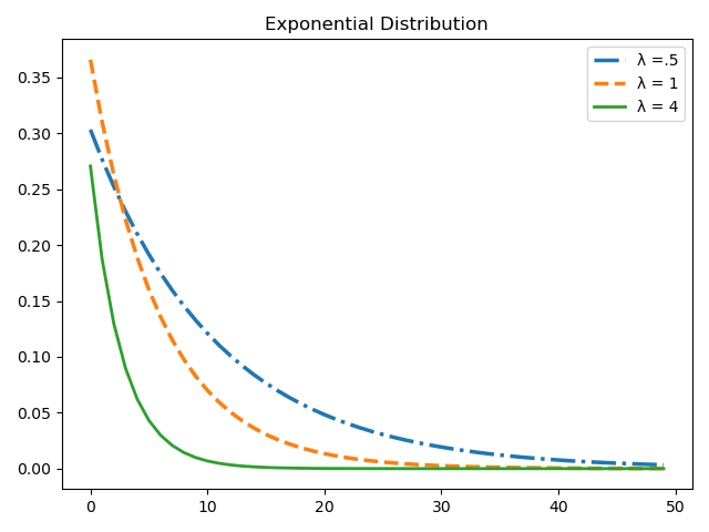
Visualizing the exponential distribution can tell us a great deal about the random variables that follow this family of distribution by change the rate parameter. In the example below, we generate a few random variables with the same mean but varying rates $\lambda$ parameters
import numpy as np
import matplotlib.pyplot as plt

x = np.linspace( 1, 10, 50 )

lambda_low = .5* np.exp( -.5 * x )
lambda_med = .9* np.exp( -.9 * x )
lambda_high = 2* np.exp( -2 * x )

plt.plot( lambda_low,  label='λ =.5', linewidth=2.5, linestyle='-.' )
plt.plot( lambda_med,  label='λ = 1', linewidth=2.5, linestyle='--' )
plt.plot( lambda_high, label='λ = 4', linewidth=2, linestyle='-' )
plt.legend()
Probability Density Function
The probability density function of the exponential distribution is given in the form below:
$$ p(x) = \begin{cases} \lambda e^{-\lambda x} & x > 0 \\ 0 & \text{ otherwise } \\ \end{cases} $$
Its to be noted that both the $x$ and $\lambda$ parameter are always positive.
Example
Suppose that the call times of customer service support follows a normal distribution with $\lambda = 1/5$.
Given that someone just called ahead of you for customer service support, what is the probability that you will
wait for 5 minutes before you are the next call?
Recall that the $scale$ argument is $\frac {1}{\lambda}$ therefore $\lambda = 5$ means $scale = \frac{1}{5}$
expon.pdf(x=5, scale=5)Expected Value
The expected value of the exponential distribution is given by the generalized formula:
$$ E(X) = \frac {1}{\lambda} $$
In the example below, we initialize a random variable with the $scale = 4$ paramater. Notice that the $\lambda = \frac {1}{4}$.
x_var = expon.rvs(scale=4, size=1000 )
x_var.mean()Variance
The variance value of the exponential distribution is given by the generalized formular:
$$ Var(X) = \frac {1}{\lambda^2}$$
x_var = expon.rvs(scale=4, size=1000 )
x_var.var()Standard Deviation
The standard deviation of the exponential distribution is the square root of the variance above.
$$ \sigma = \frac {1}{\lambda} $$
x_var = expon.rvs(scale=4, size=10000 )
x_var.std()