Gaussian Distribution
The gaussian distribution is perhaps the most well known and widely used distribution. Also known as the normal distribution, it has some nice properties that allow us to model much of the observation that we encounter naturally with data.
The normal distrbution is mathematically represented as:
$$ X \sim \mathcal{N}(\mu, \sigma) $$
where:
$\mu$: is the mean of distribution
$\sigma^2 $: is the variance of the distribution
Gaussian Random Variable
Scipy norm method provides an easy way to generate a gaussian random variable. In the example below, we generate a random variable with the $\mu = 0$ and $\sigma = 1$. Notice the following:
$loc$: The mean of the distribution
$scale$: The standard deviation of distribution
from scipy.stats import norm
norm.rvs(loc=0, scale=1, size=30)Visualizing the Random Variable
Similar to what we have seen with other distributions, we can visualize the histogram of the distribution. Below is the code to render the histogram visualization of the gaussian distribution.
import seaborn as sns

norm_rv = norm.rvs( size=10000 , loc=0, scale=1)
sns.distplot( norm_rv, kde= False, bins=20, hist_kws=dict(edgecolor="k", linewidth=1) )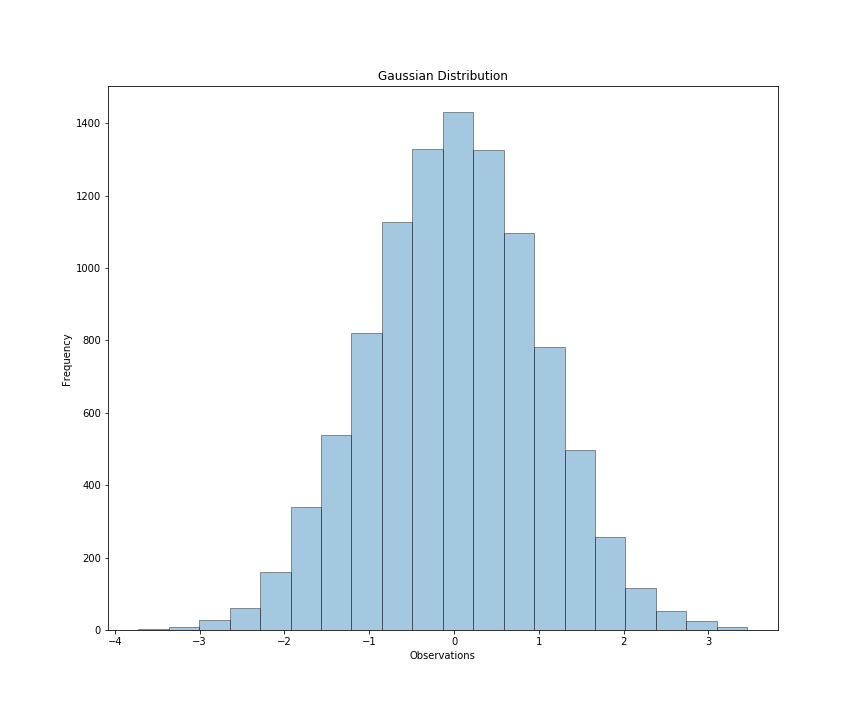
Properties of Normal Distribution
I mentioned earlier that the gaussian distribution is one of the most widely used distribution. Below are some features that make this distribution practical for modelling purposes
- Normal distributions are symmetric around their mean.
- The mean, median, and mode of a normal distribution are equal.
- 68% of the area of a normal distribution is within one standard deviation of the mean.
- Approximately 95% of the area of a normal distribution is within two standard deviations of the mean.
Probability Density Function
The probability density function is given by the formula below:
$$ P(x\ |\ \mu, \sigma^2) = \frac {1}{\sigma \sqrt{2\pi}} e^{\frac {-(x-\mu)^2}{2\sigma^2}} $$
The probability density function for the normal distribution estimates the probability of observing an estimate range of values drawn over the range provided by the normal distribution parameters.
For example, given a normal distribution centered at 5 with a standard deviation of 1, what is the probability that within a random draw, a number less than 3 is drawn.
Notice that:
$loc:$ - mean of the distribution
$scale:$ - standard deviation of the distribution
norm.pdf(x=2, loc=5, scale=1)We see that the probability of obtaining a number two from a normal distribution $X \sim \mathcal{N} (5, 1)$ is very low as expected because $2$ is more than $\sigma$ from 5.
Cumulative Density Function
The cdf of the gaussian distribution is given by the formula:
$$ P(X | \mu, \sigma^2) = \frac {1}{\sigma \sqrt{2\pi}} \int_{-\infty}^{x} e^ {\frac {-(x-\mu)^2}{2 \sigma^2}} $$
We are never really going to have to worry about the formula because python provides a much easier and intuitive
way of computing the cumulative probability.
Below, we create a normal distribution with $\mu = 3$ and $\sigma^2 = 4$ and calcuate the probability $p(x \leq
2.5 )$
norm_dist = norm( loc=3, scale=2)
norm_dist.cdf(x = 2.5)Looks just about right because $2.5$ is closer to the mean and therefore likely to be drawn form the distribution given the magnitude of $\sigma$
Expected Value
The expected value of the guassian distribution is the $\mu$. We just return the mean of the distribution. Notice that the $loc$ parameter is where we specify the mean of the normal distribution.
norm_dist = norm( loc=3, scale=2)
norm_dist.mean()Variance
We can return the variance of the distribution using the var method. As we know, var = $\sigma^2$ therefore we expect that the variance will be the square of the $scale$ parameter
norm_dist = norm( loc=3, scale=2)
norm_dist.var()Standard Deviation
Finally, the standard deviation of the normal distribution is the $\sigma$ parameter -$scale$ - we set when instantiating a normal distribution.
norm_dist = norm( loc=3, scale=2)
norm_dist.std()