Geometric Distribution

The geometric distribution is used to model the number of trials/experiments it takes for a specific event to occur - often referred to as a success. We can think about how dice rolls can we roll until number 6 is rolled. This distribution takes one parameter and models the trials needed to obtain first success.

Mathematical representation:

$$ X \sim {Geometric}(p)$$

where:
$p$: is the probability of success.

A few conditions must be true for the geometric distribution to hold:

1. Each trial has binary outcomes
2. All trials have the same probability of success
3. Each trial is independent of the previous trial

Geometric Random Variable

To generate a random variable that is geometrically distributed, we call the geom method and initialize the probability value. Notice that the output is a set of integers that are the number of trails needed for yielding a success event given the probability.

from scipy.stats import geom

geom_dist = geom.rvs(p=.3, size=100)
geom_dist

array( [1, 2, 3, 1, 1, 1, 1, 1, 3, 6, 3, 7, 1, 2, 8, 3, 5, 2, 1, 19, 1, 5, 7, 3, 1, 1, 6, 1, 1, 5, 2, 3, 4, 2, 1, 4, 1, 3, 3, 1, 2, 11, 9, 5, 4, 8, 2, 12, 3, 9, 1, 1, 4, 2, 4, 5, 4, 1, 8, 1, 1, 7, 1, 6, 4, 7, 1, 1, 1, 4, 2, 1, 5, 3, 5, 5, 3, 9, 1, 4, 10, 2, 3, 1, 6, 2, 6, 2, 11, 10, 1, 2, 1, 3, 1, 5, 1, 1, 6, 2])

Visualizing the Distribution

We can visualize the random variable we generated above. We notice that the probability of success decreases as the number of trials increases.

geom_dist = geom.rvs(p=.3, size=1000)
_ = plt.hist(geom_dist, bins=20, ec='black')
plt.xlabel('Geometric Trials')
plt.ylabel('Frequency')
plt.title('Geometric Distribution')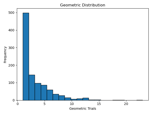

Probability Mass Function

The probability mass function of the geometrics distributions is a slight modification to the binomial distribution.

$$f_X(x) = p(1-p)^{x-1}$$

where:
$x$: number of trials until the first success

Example:
Suppose the probability of getting a correct answer from a set of random questions is .3. What is the probability of getting the correct answers in the first 5 questions?

geom_dist = geom(p=.3)
geom_dist.pmf(5), .3*(1-.3)**(5-1)

(0.07202999999999998, 0.07202999999999998)

Probability Density Function

The probability density function returns the cumulative probability of success. For example, to compute the probability of success after the first 5 trials, we can run the following method.

geom_dist.cdf(5)

0.83193

Expected Value

The expected value of the geometric distribution is given by:

$$ E(X) = \frac {1}{p} $$

where:
$p$: is the probability of success

In python, to compute the expected value from the geometric distribution, we can use the formula or the mean method

geom_dist = geom( p=.3 )
geom_dist.mean(), 1/.3

(3.3333333333333335, 3.3333333333333335)

Variance

The variance of the geometric distribution can be calculated with the following formular:

$$ Var(X) = \frac {1-p}{p^2}$$

The distribution object has the variance method but we can also compute the variance with the formula.

geom_dist.var(), (1-.3)/(.3**2) 

(7.777777777777779, 7.777777777777778)

Standard Deviation

The standard deviation is simply the square root of variance. For the geometric distribution, the standard deviation is computed as:

$$ sigma = \frac { \sqrt {1 - p} } {p} $$

Computing this in python assuming that $p$ = .3:

geom_dist.std(), np.sqrt(1-.3)/.3

(2.7888667551135855, 2.7888667551135855)