Equal Probability and Law of Large Numbers
In the previous section we briefly discussed the fair coin. Notice that for the fair coin flip, we essentially are saying that there is a 50% chance that heads will turn up. However, it important to distinguish the probability and exact occurrence of heads.
To do this, we will run a simulation of flipping the coin k times and compute the exact times. Below is the python implementation of the simulation:
import numpy as np
import matplotlib.pyplot as plt

def coin_flip_simulation(n_simulations):
    """
    This function will random select between 1 and -1
    1: Heads
    -1: Tails
    params:
        n_simulations: number of experiments i.e. coin flips

    returs:
        returns the value counts of the simulated results
    """
    coin_flips = np.array(2*(np.random.rand(n_simulations)>.5)-1)

    return np.unique(coin_flips, return_counts=True)
Now let's test the results for 1000 simulations
events, occurrences = coin_flip_simulation(1000)
print(events), print(occurrences)We notice that the number of heads -1 is higher than the number of tails -1. Based on our information about a fair coin, we know that the probability of heads is 50% but we see that we do not get 500 heads in 1000 flips. Let's try and simulate the flips across k samples groups with n experiments in each group.
Higher Sampling and Multi-Sampling
To illustrate the law of large numbers, let's take 100 groups each with 1000 sampling simulation and sum the results together. We then plot the histograms to view the distribution of the sums ( which should be centered around zero given both 1 and -1 have 50% probability of occurrence).
def multiple_simulation(n_simulations, k_groups):
    """This function will execute multiple simulations"""

    flip_matric = 2*(np.random.rand(n_simulations, k_groups)>.5)-1
    value_sums = np.sum(flip_matric, axis=0)

    return value_sums

def histogram_plot(k_1, k_2, k_3):
    """  """

    set_1 = multiple_simulation(10000, k_1)
    set_2 = multiple_simulation(10000, k_2)
    set_3 = multiple_simulation(10000, k_3)


    fig = plt.figure(figsize=(15,5))
    fig.add_subplot(131)
    plt.hist(set_1,20, ec='black')
    plt.title('K= {} groups, N= 10000 simulations'.format(k_1))

    fig.add_subplot(132)
    plt.hist(set_2,20, ec='black')
    plt.title('K= {} groups, N= 10000 simulations'.format(k_2))

    fig.add_subplot(133)
    plt.hist(set_3, 20,ec='black')
    plt.title('K= {} groups, N= 10000 simulations'.format(k_3))
    plt.show()

    return "Histogram Plot"
histogram_plot(10, 100, 1000)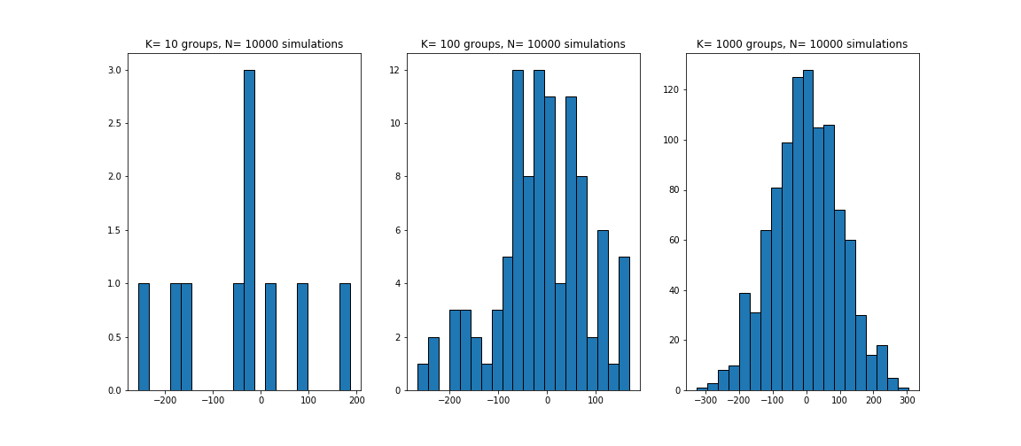
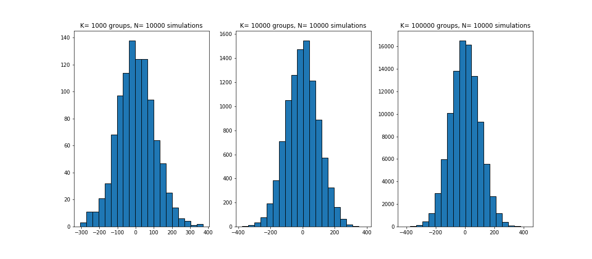
Even Higher Multi-Samples
As seen above, the convergence of the coin simulation is not as clearly observable even with 10000 coin flips across 200 sampling groups. But as the number of simulations increases, we see that the sum of heads and tails converges to a distribution centered at zero
histogram_plot(1000, 10000, 100000)