Poisson Distribution

The poisson distribution models the probability of random events ( random variable ) that happen within a given time interval. For example, the number of children born every hour can likely be modelled with the poisson distribution.

Mathematically, the poisson distribution is symbolized as:

$$ X \sim Poisson_{\lambda}$$

where:
$\lambda$: is the expected value/rate of events of the random variable.

More generally, the poisson distribution models a random variable whose:

1. Events can be counted within the time interval
2. The rate of events is established/known within the interval
3. Events are independent with each other within the time interval

Poisson Random Variable

As we see above, the poisson distribution takes on a parameter which is the rate of events $\lambda$. The resulting output is the count of observations that are drawn from a poisson distribution with the specified $\lambda$ value - in this case $2.5$.

from scipy.stats import poisson

poisson_rv = poisson.rvs(2.5, size=100)
poisson_rv

array([2, 3, 3, 4, 5, 3, 5, 3, 3, 2, 0, 2, 2, 5, 3, 2, 3, 2, 5, 0, 2, 0, 3, 3, 4, 2, 2, 2, 5, 5, 0, 2, 3, 5, 2, 1, 2, 2, 2, 3, 0, 1, 3, 5, 3, 3, 3, 4, 2, 3, 0, 2, 2, 5, 3, 1, 2, 1, 1, 5, 1, 3, 2, 1, 3, 1, 1, 3, 1, 4, 3, 2, 4, 3, 2, 4, 3, 3, 1, 2, 2, 2, 1, 1, 1, 4, 4, 4, 3, 2, 3, 4, 3, 3, 5, 2, 4, 2, 5, 1])

Visualizing the Poisson Distribution

To help visualize the poisson distribution, we use a combination of possible events from the probability mass function to demonstrate the shape of the poisson distribution based on different $\lambda$ parameters. We do this at:

$\lambda$ = 10
$\lambda$ = 5
$\lambda$ = 1

import numpy as np
import matplotlib.pyplot as plt
from scipy.special import factorial

# Event Counts
x = np.arange(0, 30, 1)

poisson_rv_1 = ((10**x)*np.exp(-10))/factorial(x, exact=True)
poisson_rv_2 = ((5**x)*np.exp(-5))/factorial(x, exact=True)
poisson_rv_3 = ((2**x)*np.exp(-2))/factorial(x, exact=True)

plt.plot(x, poisson_rv_1, label='λ = 10', linewidth=2.5, linestyle='-')
plt.plot(x, poisson_rv_2, label='λ = 5', linewidth=2.5, linestyle='--')
plt.plot(x, poisson_rv_3, label='λ = 2', linewidth=2.5, linestyle='-')
plt.title('Poissob Distriubtion with Varying λs')
plt.xlabel('K Counts')
plt.ylabel('Probabilities')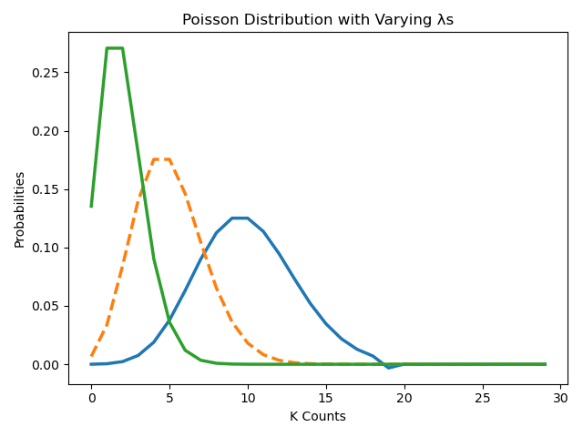

Notice the shape of the distribution as the $\lambda$ increases. The distribution center moves to the right and the variance increases with higher $lambda$ values.