Uniform Distribution
The uniform distribution is characterized by equal probability across all possible events on the sample space. For example, what is the probability of picking a number between 10 and 20. This kind of problem can be modeled using a uniform distribution.
Mathematically:
$$ X \sim Uniform_{a, b}(p) $$
where:
$a$: lower bound for the interval space
$b$: upper bound for the interval space
Uniform Random Variable
The uniform distribution takes 2 parameters representing the upper and lower bound of the distribution. Below we construct a random variable with values between $0$ and $10$. Notice that scale value is the difference $b-a$ while loc is the lower bound value $a$.
from scipy.stats import uniform

uniform_rv = uniform.rvs( size=30 , loc=10, scale=21)
uniform_rvVisualizing the Distribution
We can visualize the random variable we generated above with seaborn's distribution plot plot that returns the frequency counts of all observations.
Notice that the scale is the difference $b-a$ while loc is lower bound value $a$ parameter
uniform_rv = uniform.rvs( size=10000 , loc=10, scale=10)
sns.distplot( uniform_rv, kde= False, bins=10 )
plt.title('Uniformly Distributed')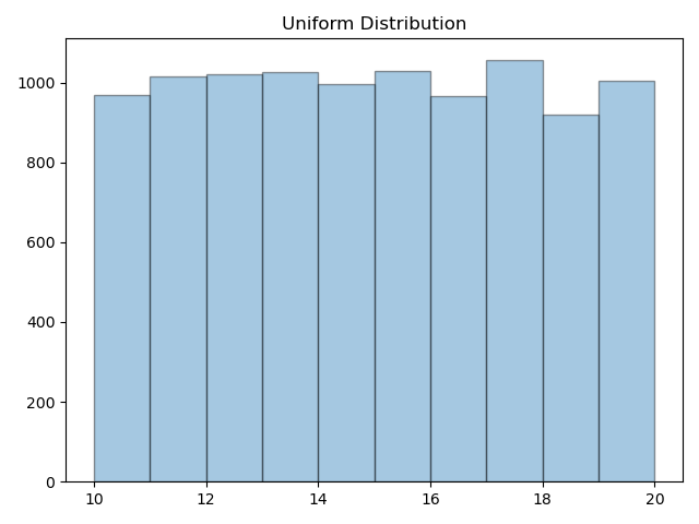
Probability Density Function
We can compute the probability of a uniform distribution using the functional form below:
$$ p(x) = \begin{cases} 0 & \text{ for } x < a \\ \frac {1}{b-a} & \text{for } a \leq x \leq b \\ 0 & \text{ for } x > b \end{cases} $$
Below is an example of how to compute the probability density with lower and upper bounds at $10$ and $20$.
uniform_dist = uniform(loc=10, scale=10)
uniform_dist.pdf( x=15 ), 1/(20-10)Since we know that the distribution has uniform probability, we expect every input value for x in the pdf method will return the same probability.
Cumulative Distribution Function
On the other hand, the cumulative distribution function returns the collective probability based on on the lower and upper bounds of the distribution.
Mathematically we express the cdf as:
$$ p(x) = \begin{cases} 0 & \text{ for } x < a \\ \frac {x-a}{b-a} & \text{for } a \leq x \leq b \\ 0 & \text{ for } x > b \end{cases} $$
Below, I demonstrate that using both formula and the cdf function will return the same result for the variance. We need to provide an x value relative to the distribution.
uniform_dist.cdf(x=15), (15-10)/(20-10)Expected Value
The expected value of the uniform distribution is given by the formula
$$ \mathbb{E}(X) = \frac {1}{2} (a + b) $$
As we have seen before, we can compute the expected value by returning the mean.
uniform_dist.mean(), (20 + 10)/2Variance
The variance of the uniform distribution is mathematically expressed as:
$$ Var(X) = \frac {1}{12}(b-a)^2$$
Compute the variance using either methods will return the same value.
uniform_dist.var(), (1/12)*(20-10)**2Standard Deviation
The standard of the uniform distribution is mathematically expressed as:
$$ \sigma = \sqrt { \frac {1}{12}} (b-a) $$
To compute the value in python, we use both the formula and std method
uniform_dist.std(), np.sqrt(1/12)*(20-10)