Fitting Regression Trees

Following the previous implementation of Decision Trees Classifier, this note covers the implementation of Decision Trees Regression.

# loading the necessary libraries
# keep in mind that some libraries need installing
library(ISLR)         
library(ggthemr)
library(ggplot2)
library(tidyverse)
library(tidymodels)
library(rpart.plot)
# loading the ames dataset
data("ames")
head(ames, n=10)
OUTPUT# A tibble: 5 × 74 MS_SubClass MS_Zoning Lot_Frontage Lot_Area Street 1 One_Story_1946… Resident… 141 31770 Pave 2 One_Story_1946… Resident… 80 11622 Pave 3 One_Story_1946… Resident… 81 14267 Pave 4 One_Story_1946… Resident… 93 11160 Pave 5 Two_Story_1946… Resident… 74 13830 Pave # ℹ 69 more variables: Alley , Lot_Shape , # Land_Contour , Utilities , # Lot_Config , Land_Slope , # Neighborhood , Condition_1 , # Condition_2 , Bldg_Type , # House_Style , Overall_Cond , # Year_Built , Year_Remod_Add , …

The response variable from the dataset is the Sale_Price. As see on the data overview, there are a number of variables/features that are part of the dataset. We will fit all of these features into the Tree Model.

# for reproducibility
set.seed(5672)

ames_split <- initial_split(ames, prop = .8)

# training datasets
train_data <- training(ames_split)
test_data <- testing(ames_split)

dim(train_data); dim(test_data);
OUTPUT[1] 2344 74 [1] 586 74
# fitting a regression
decision_tree_regression <-  decision_tree() %>%
                             set_engine("rpart") %>%
                             set_mode("regression")
# fitting a regression tree
reg_tree_fit <- fit(decision_tree_regression, data = train_data, formula =  Sale_Price ~ .)

reg_tree_fit
OUTPUTparsnip model object n= 2344 node), split, n, deviance, yval * denotes terminal node 1) root 2344 1.534682e+13 181783.8 2) Garage_Cars< 2.5 2025 6.031772e+12 161560.3 4) Neighborhood=North_Ames,Old_Town,Edwards,Sawyer,... 1146 1.514126e+12 131477.7 8) Gr_Liv_Area< 1324.5 709 5.426151e+11 118965.3 16) Neighborhood=Old_Town,Edwards,Brookside,... 334 2.256970e+11 102979.9 * 17) Neighborhood=North_Ames,Sawyer,Mitchell,Northpark_Villa,Blueste,Landmark 375 1.555519e+11 133203.1 * 9) Gr_Liv_Area>=1324.5 437 6.804199e+11 151778.1 * 5) Neighborhood=College_Creek,Somerset,Northridge_Heights,Gilbert,... 879 2.128450e+12 200780.7 10) Gr_Liv_Area< 1482.5 365 3.987556e+11 170827.7 * 11) Gr_Liv_Area>=1482.5 514 1.169682e+12 222050.8 22) Total_Bsmt_SF< 959.5 232 2.037570e+11 196162.6 * 23) Total_Bsmt_SF>=959.5 282 6.825210e+11 243348.9 * 3) Garage_Cars>=2.5 319 3.229479e+12 310161.3 6) Neighborhood=North_Ames,College_Creek,Old_Town,Edwards,... 164 8.653521e+11 254133.3 12) Year_Remod_Add< 1989.5 24 4.316782e+10 153937.5 * 13) Year_Remod_Add>=1989.5 140 5.399394e+11 271309.7 * 7) Neighborhood=Northridge_Heights,Northridge,Stone_Brook,Veenker 155 1.304597e+12 369442.5 14) First_Flr_SF< 2217 142 7.760310e+11 353747.8 28) Gr_Liv_Area< 2647.5 115 3.136169e+11 331498.0 * 29) Gr_Liv_Area>=2647.5 27 1.629962e+11 448515.9 * 15) First_Flr_SF>=2217 13 1.115215e+11 540876.9 *

Pruning Complexity Parameter

The rpart engine performs a range of cost complexity assessments even with the base model. It performs a 10-fold CV by default. The plotcp() method provides us with the visualization of the validation and a way to choose the number of terminal nodes to use. In the visualization below, 11 nodes seem to be best performing.

reg_tree_fit %>% 
    extract_fit_engine() %>% 
    plotcp()
Best Fit Decision Tree Regression

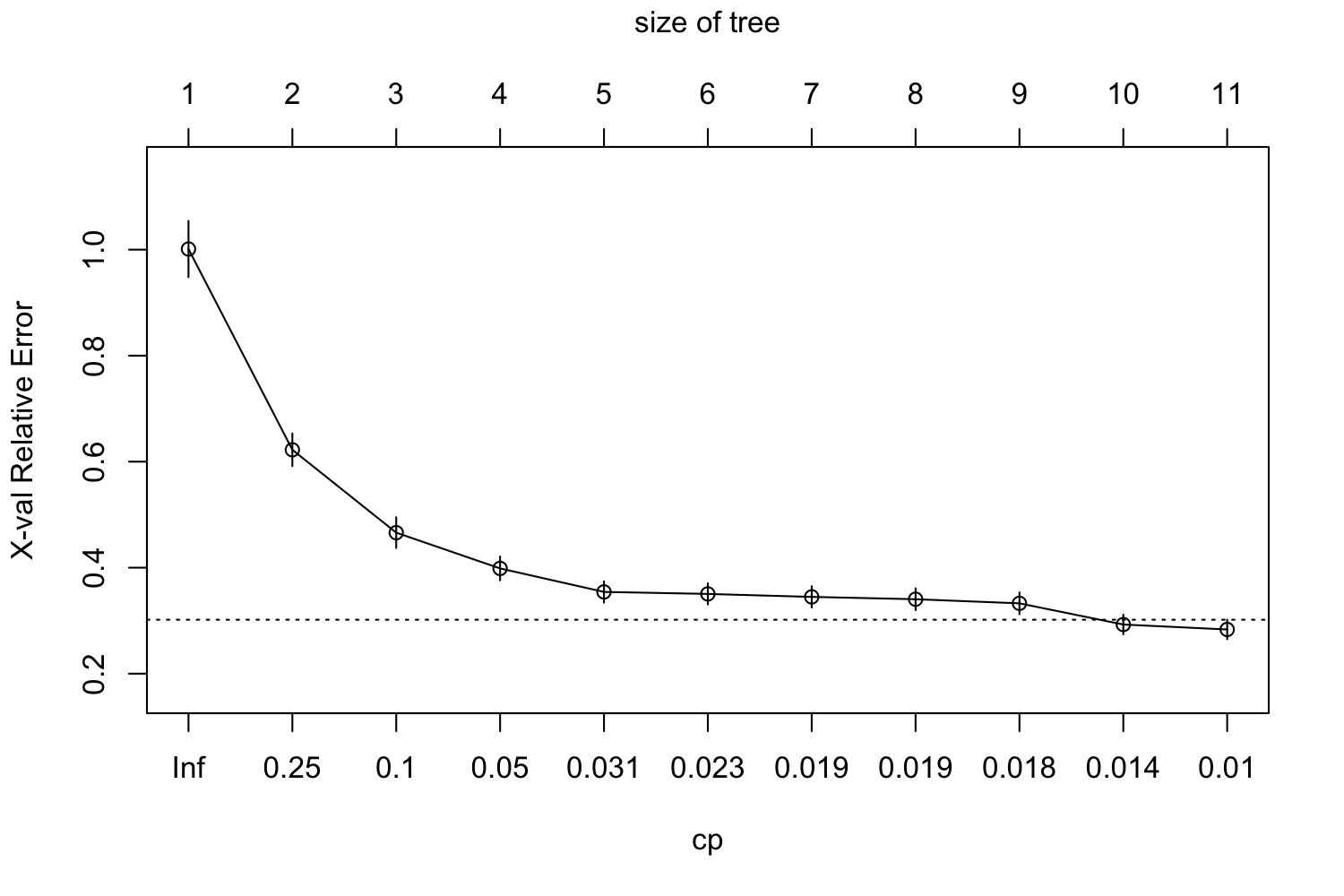
Model Fit Assessment and Tree Visualization

As this is a regression task, we can extract regression model assessment metrics such as rmse to the dataset.

# showing the top predicted values
augment( reg_tree_fit, new_data = train_data ) %>%
    rmse( truth = Sale_Price, estimate = .pred )
OUTPUT# A tibble: 1 × 3 .metric .estimator .estimate 1 rmse standard 38741.
reg_tree_fit %>% 
  extract_fit_engine() %>% 
  rpart.plot(roundint = FALSE) 
Best Fit Decision Tree Regression

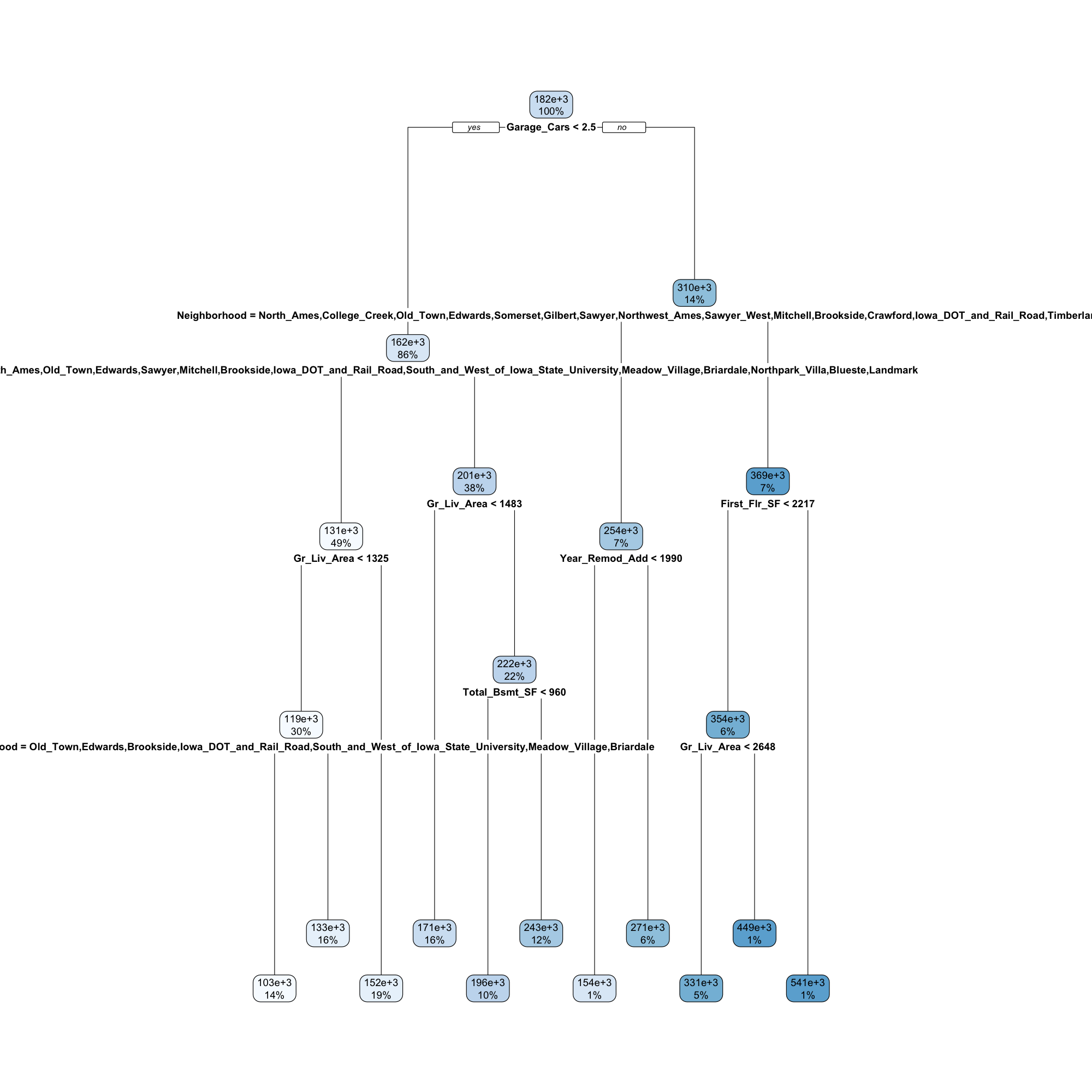
Predictions on Test and New Observations

We can then run predictions on the test data set and/or new observation in the same way we have with the train set above.

augment( reg_tree_fit, new_data = train_data ) %>%
    rmse( truth = Sale_Price, estimate = .pred )
OUTPUT# A tibble: 1 × 3 .metric .estimator .estimate 1 rmse standard 38741.