Lasso Regression

Lasso Regression, short for Least Absolute Shrinkage and Selection Operator, is another powerful regularization technique used in linear modeling. Like Ridge Regression, Lasso introduces a penalty to the regression model to prevent overfitting and manage multi-collinearity. However, the key difference lies in the nature of the penalty applied.

In Lasso Regression, the penalty added to the objective function is based on the absolute values of the coefficients (known as the L1 norm), as opposed to the squared coefficients used in Ridge Regression (L2 norm). Furthermore, the Lasso Penalty imposes it's impact by forcing coefficients of variables that are small to zero, thereby eliminating insignificant features.

$$ $$

Because we have seen how to implement Ridge regression, we will now demonstrate implementation of Lasso Regression. We will skip some ideas already covered earlier in the note.

Implementation of Lasso Regression on Hitter's Dataset

library(ISLR2)
library(tidyverse, quietly = TRUE)

hitters <- as_tibble(Hitters) %>% 
            filter( !is.na(Salary) )
dim(hitters)

OUTPUT[1] 263 20

Define the Lasso Regression Model

In this example, we first define the Lasso recipe, model and then define a workflow to implement the model

Lassa Recipe

This recipe simply defines the formular of our regression model.

lasso_recipe <- 
  recipe(formula = Salary ~ ., data = train_data) %>% 
  step_novel(all_nominal_predictors()) %>% 
  step_dummy(all_nominal_predictors()) %>% 
  step_zv(all_predictors()) %>% 
  step_normalize(all_predictors())

OUTPUT── Recipe ───────────────── ── Inputs Number of variables by role outcome: 1 predictor: 19 ── Operations • Novel factor level assignment for: all_nominal_predictors() • Dummy variables from: all_nominal_predictors() • Zero variance filter on: all_predictors() • Centering and scaling for: all_predictors()

Lasso Model

Now we implement the Lasso model by setting the variable mixture = 1

lasso_spec <- 
  linear_reg(penalty = tune(), mixture = 1) %>% # mixture 1 for L1 - Lasso penalty
  set_mode("regression") %>% 
  set_engine("glmnet") 

lasso_spec

OUTPUTLinear Regression Model Specification (regression) Main Arguments: penalty = tune() mixture = 1 Computational engine: glmnet

Lasso Regression Workflow

We can now complete the model into a workflow

lasso_workflow <- workflow() %>% 
  add_recipe(lasso_recipe) %>% 
  add_model(lasso_spec)

lasso_workflow

OUTPUT══ Workflow ══════════════════════════════════════════════════ Preprocessor: Recipe Model: linear_reg() ── Preprocessor ────────────────────────────────────────────── 4 Recipe Steps • step_novel() • step_dummy() • step_zv() • step_normalize() ── Model ───────────────────────────────────────────────────── Linear Regression Model Specification (regression) Main Arguments: penalty = tune() mixture = 1 Computational engine: glmnet

In the Ridge regression, we saw the implementation of a workflow for indiviual models without grid search. Here, we go directly to using grid search by generating different values of the penalty

penalty_grid <- grid_regular(penalty(range = c(-2, 2)), levels = 50)
penalty_grid

OUTPUT# A tibble: 50 × 1 penalty 1 0.01 2 0.0121 3 0.0146 4 0.0176 5 0.0212 6 0.0256 7 0.0309 8 0.0373 9 0.0450 10 0.0543 # ℹ 40 more rows # ℹ Use print(n = ...) to see more rows

tune_grid - Hyperparameter search

We can no perform a grid search on the different parameters of lambda for our Lasso Regression using the tune_grid() function

tune_res <- tune_grid(
  lasso_workflow,
  resamples = hitters_fold, 
  grid = penalty_grid)

library(ggthemr)
ggthemr('fresh')
autoplot(tune_res)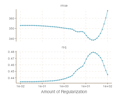

Select best performing parameter with select_best()

Again, we see mixed effects of the metrics with each lasso penalty. We can then extract the best model using the select_best()

best_penalty <- select_best( tune_res, metric = "rsq" )

lasso_final <- finalize_workflow(lasso_workflow, best_penalty)

lasso_final_fit <- fit(lasso_final, data = train_data)

OUTPUT══ Workflow [trained] ══════════════════════════════════════════════════ Preprocessor: Recipe Model: linear_reg() ── Preprocessor ──────────────────────────────────────────────────────── 4 Recipe Steps • step_novel() • step_dummy() • step_zv() • step_normalize() ── Model ─────────────────────────────────────────────────────────────── Call: glmnet::glmnet(x = maybe_matrix(x), y = y, family = "gaussian", alpha = ~1) Df %Dev Lambda 1 0 0.00 256.200 2 1 5.30 233.500 3 1 9.70 212.700 4 1 13.35 193.800 5 3 18.03 176.600 6 3 22.51 160.900 7 3 26.22 146.600 8 4 29.30 133.600 9 4 31.87 121.700 10 4 34.01 110.900 11 4 35.78 101.100 12 4 37.25 92.080 13 5 38.52 83.900 14 5 39.96 76.450 15 6 41.35 69.660 16 6 42.52 63.470 17 6 43.49 57.830 18 6 44.30 52.690 19 6 44.97 48.010 20 6 45.52 43.750 21 6 45.98 39.860 22 6 46.37 36.320 23 6 46.68 33.090 24 6 46.95 30.150 25 6 47.17 27.470 26 6 47.35 25.030 27 7 47.50 22.810 28 8 47.63 20.780 29 8 47.73 18.940 30 9 47.83 17.250 31 9 47.94 15.720 32 10 48.04 14.330 33 10 48.13 13.050 34 10 48.20 11.890 35 10 48.26 10.840 36 11 48.44 9.874 37 12 48.72 8.997 38 13 49.20 8.197 39 14 50.00 7.469 40 14 50.72 6.806 41 14 51.24 6.201 42 14 51.72 5.650 43 15 52.08 5.148 44 15 52.47 4.691 45 16 52.73 4.274 46 16 53.02 3.894 ... and 29 more lines.

augment(lasso_final_fit, new_data = test_data) %>%
  rsq(truth = Salary, estimate = .pred)

OUTPUT# A tibble: 1 × 3 .metric .estimator .estimate 1 rsq standard 0.491