Ridge Regression
The Ridge Regression method is a regularization technique that imposes a penalty on predictors with a significant large parameter. By adding a tuning parameter, $\lambda$ to the objective function, ridge regression imposes a penalty for large coefficients forcing the overall effect to zero in order to minimize the objective function (and vice versa).
To motive Ridge regression, let's reconstruct the loss function/objective function for regression by adding the weights. Mathematically, we can think of it this way:
$$ RSS(w) + \lambda||W||_2^2 $$
where $RSS$ is the residual sum of squares, $\lambda$ is the ridge hyper parameter
What happens when:
$\lambda$ = 0, then the total cost is $RSS(W)$ which is the original least squares formulation of linear regression
$\lambda = \infty$, the only minimizing solution is when $\hat W$ = 0, because the the total $RSS(W) = 0$.
Then the ridge solution is always between $0 \le ||W||_2^2 \le RSS(W)$
Now that we have explore conceptually the idea, we move on to implementation.
Implementation of Ridge Regression with Hitter's Dataset
In the note below, we implement ridge regression using tidymodels. Specifically, we will need the
library(ISLR2)
library(tidyverse, quietly = TRUE)

hitters <- as_tibble(Hitters) %>%
            filter( !is.na(Salary) )
dim(hitters)Defining the Ridge Regression Model
As we have done several times on the lab, we begin by
# install.packages("glmnet")
library(tidymodels, quietly = TRUE)

ridge_regression <- linear_reg( mixture = 0, penalty = 0 ) %>%  # setting a rigde penalty of zero
                    set_mode("regression") %>%
                    set_engine("glmnet")

ridge_regressionWe have not defined the specification for the ridge regression model. We can go ahead and fit the model using the data. For this modeling process, we skip the train and test splitting. This knowledge is expected. Instead, we focus on the implementation details.
ridge_regression_fit <- fit( ridge_regression, Salary ~ ., data = hitters )

ridge_regression_fit %>% tidy()The output above shows what the estimate of the variable parameter is when rigde penalty is set to zero (no penalty). However, we can see the results when the ridge penalty is increased. Not that we may need a sufficiently high ridge penalty to see the changes in the estimated coefficient. In the case below, we use 1000.
tidy(ridge_regression_fit, penalty = 1000)Try a few penalty values for yourself now. What do you see as the result?
Visualizing Impact of Penalty
Using
par(mar = c(5, 5, 5, 1))
ridge_regression_fit %>%
  parsnip::extract_fit_engine() %>%
  plot(xvar = "lambda")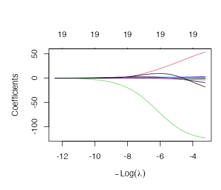
Tuning the Ridge L2 Penalty
We have seen that we can implement various penalty values for the same model. This is well and good for demonstration by in reality, we need a way to optimize the L2 parameter. In the next section, we demonstrate how to build a pipeline that finds the best penalty value for us.
We begin by splitting the data into train and test and then create a cross-validation set.
set.seed(1234)
hitters <- as_tibble(ISLR2::Hitters) %>% drop_na()

names(hitters)data_split <- initial_split(hitters, strata = "Salary")
train_data <- training(data_split)
test_data <- testing(data_split)
hitters_fold <- vfold_cv(train_data, v = 10)
hitters_foldTune Grid for Parameter Search
We can now use the tune_grid() function to perform hyperparameter turning using grid search. To do this, we need to create a workflow, samples and output file to contain the parameters. Before we do this, we will need to perform data processing as ridge regression is sensitive to scale. For this, we will normalize the data.
ridge_recipe <- recipe( formula = Salary ~ ., data = train_data ) %>%
                step_novel( all_nominal_predictors() ) %>% # Handle new (unseen) factor levels in categorical predictors
                step_dummy( all_nominal_predictors() ) %>% # Convert all categorical predictors to dummy/indicator variables
                step_zv( all_predictors() ) %>%            # Remove predictors with zero variance (constant variables)
                step_normalize( all_predictors() )         # Normalize (center and scale) all predictors to have a mean
                                                                                 # of 0 and standard deviation of 1

ridge_recipeWith the pre-processing above complete, we can now create the model specification. This time, we set the penalty to
ridge_spec <- linear_reg( penalty = tune(), mixture = 0 ) %>%
        set_mode("regression") %>%
        set_engine("glmnet")

ridge_specridge_workflow <- workflow() %>%
add_recipe( ridge_recipe ) %>%
add_model( ridge_spec )
ridge_workflowFinally, the last thing we need is the values of the penalty we are going to pass on to the grid search. We can
provide these range of values in many forms. One of the forms is using
penalty_grid <- dials::grid_regular(
  x = dials::penalty(
    # Define the range of the penalty parameter.
    range = c(-5, 5),
    # Apply a logarithmic transformation (base 10) to the penalty values.
    trans = scales::log10_trans()
  ),
  # Create 50 evenly spaced levels within the specified penalty range.
  levels = 50
)

penalty_grid %>% slice_head( n = 10)Note that the values here are scaled to meet the normalization step we performed on the dataset.
Tuning the Parameter
Now we have everything we need. We can go ahead and implement the grid search.
tune_res <- tune::tune_grid(
  object = ridge_workflow,    # object with ridge model
  resamples = hitters_fold,   # define cross-validation fold
  grid = penalty_grid        # testing penalty values
)

tune_resWe see that our cross validation is complete. We can immediately look at the cross-validation plot output to gauge the impact of regularization on the data.
autoplot(tune_res)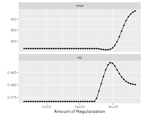
From the plot we see that early regularization have limited impact on rsq and rmse. However, over time we see the impact on the metrics with rsq as the penalty increases. This is also the case for rsme metric as well.
Overall Metrics
We can capture the metrics for the regularization grid search by passing the
collect_metrics(tune_res)To get the best penalty, we can simply use the select_best which takes on the grid_search objects and a parameter
to select for the best results. The example below uses
best_penalty <- select_best(tune_res, metric = "rsq")
best_penaltyFinally, we can then extract the final penalization and retrieve the model fit.
ridge_final <- finalize_workflow( ridge_workflow, best_penalty )

ridge_final_fit <- fit(ridge_final, data = train_data)
Now, we apply this to the testing data.
augment(ridge_final_fit, new_data = test_data) %>%
  rsq(truth = Salary, estimate = .pred)