Log Transformation
Log Transformation is a effective transformation typically applied on variables with large scales such as prices of a home. The fundamental idea, particularly in regression, of using the Log Transformation is to convert the data from its original distribution to a normal distribution by dealing with skews. This is of course important for linear regression which has assumptions about errors.
Let's look at an example using the Ames Housing Dataset
# loading data processing and visualization theme
library(tidyverse)
library(ggthemr)

# loading a visualization them
ggthemr('fresh')
ames <- as_tibble(read.csv("../Datasets/ames.csv"))
head(ames)| Order | PID | area | price | MS.SubClass | MS.Zoning | Lot.Frontage |
|---|---|---|---|---|---|---|
| 1 | 526__301__100 | 1,656 | 215,000 | 20 | RL | 141 |
| 2 | 526__350__040 | 896 | 105,000 | 20 | RH | 80 |
| 3 | 526__351__010 | 1,329 | 172,000 | 20 | RL | 81 |
| 4 | 526__353__030 | 2,110 | 244,000 | 20 | RL | 93 |
| 5 | 527__105__010 | 1,629 | 189,900 | 60 | RL | 74 |
| 6 | 527__105__030 | 1,604 | 195,500 | 60 | RL | 78 |
Let's visualize the response variable: Sales Price
ames %>%
  ggplot(., aes(x = price)) +
  geom_histogram( color = 'black', bins = 30 ) +
  ggtitle("Distribution of Sale Price")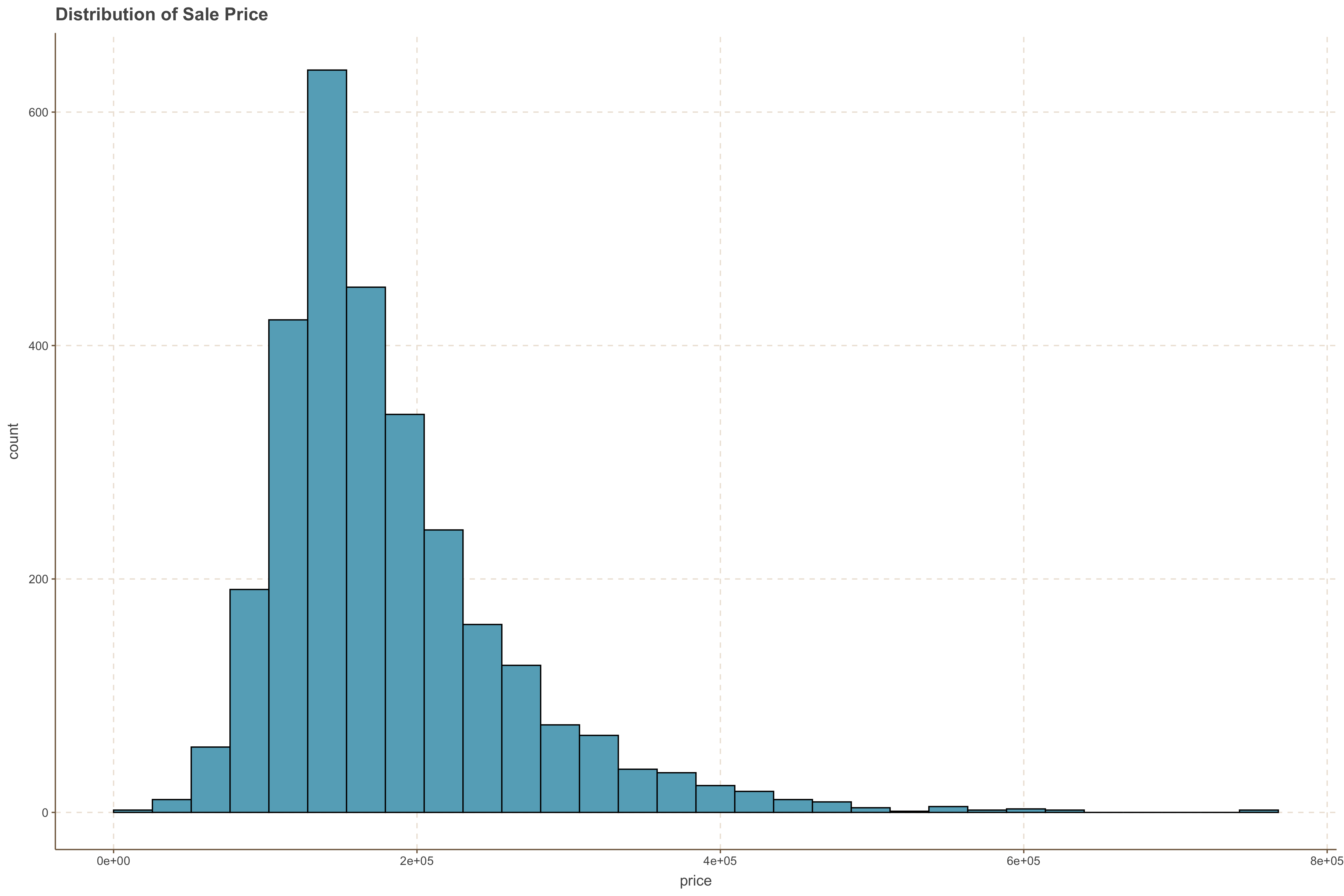
ames %>%
  ggplot(., aes(x = log(price))) +
  geom_histogram( color = 'black', bins = 30 ) +
  ggtitle("Distribution of Log Sale Price")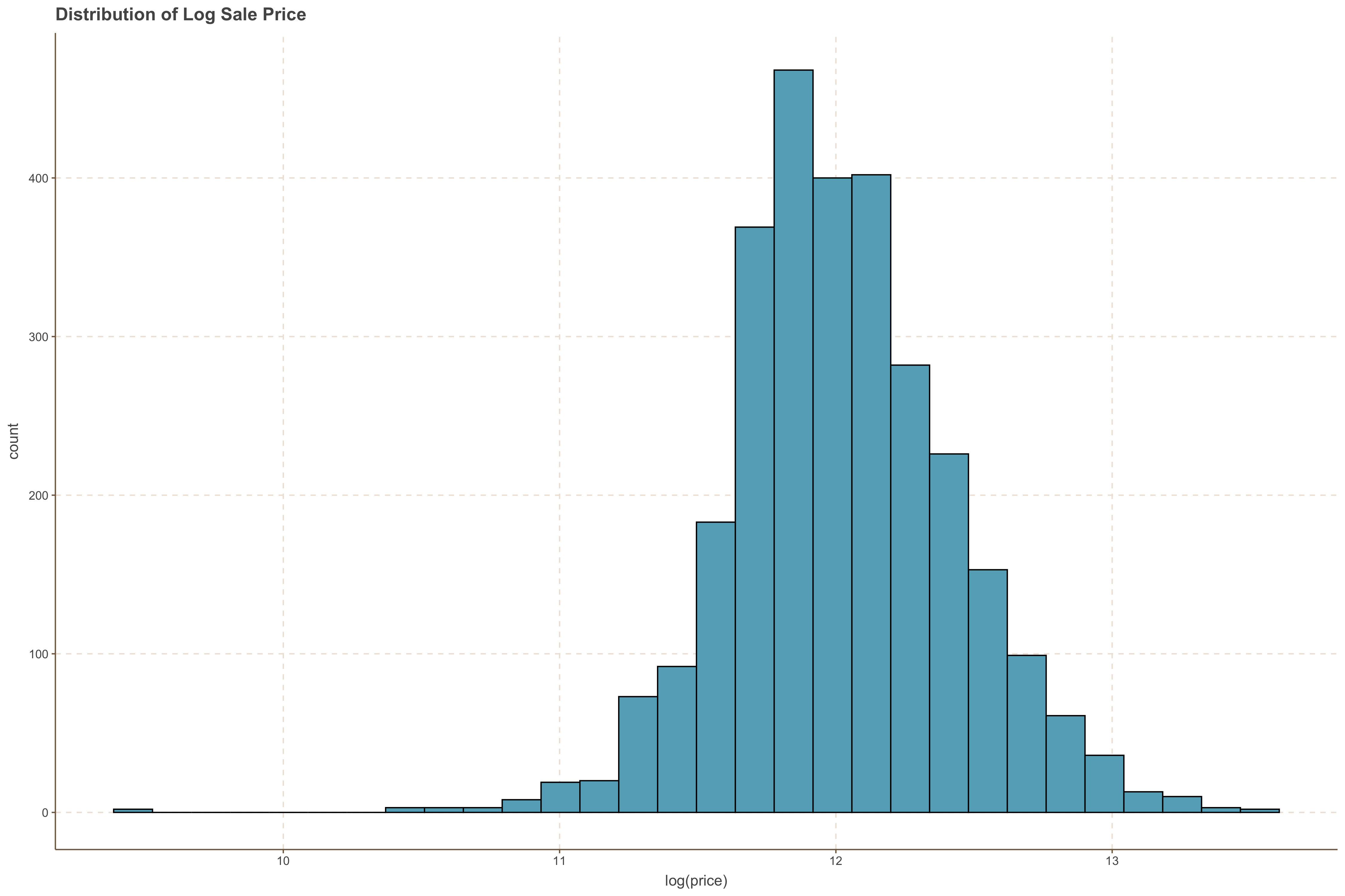
We notice that the data is much closer to a normal distribution now however, we see that the log transformation has introduced a left skew.
Box-Cox Transformation
Another alternative is the Box-Cox Transformation which aims to achieve similar results as the log transformation but converting the data into a normal distribution. The Box-Cox transformation is particularly useful with non-normal data. The formal definition is given as:
$$ Y(\lambda) = \begin{cases} \frac{Y^\lambda - 1}{\lambda} & \text{if } \lambda \neq 0 \\ \ln(Y) & \text{if } \lambda = 0 \end{cases} $$
where $\lambda$ is a parameter that is estimated from the data, determining the exact nature of the transformation. The Box-Cox transformation adjusts the data such that it approximates a normal distribution, which is beneficial for many statistical modeling techniques that assume normality of the input data.
Let's see how to implement it. We first compute the lambda parameter and transform the variable with the function above.
library(forecast)
# computing the lambda parameter
boxcox_lambda <- BoxCox.lambda(ames$price)
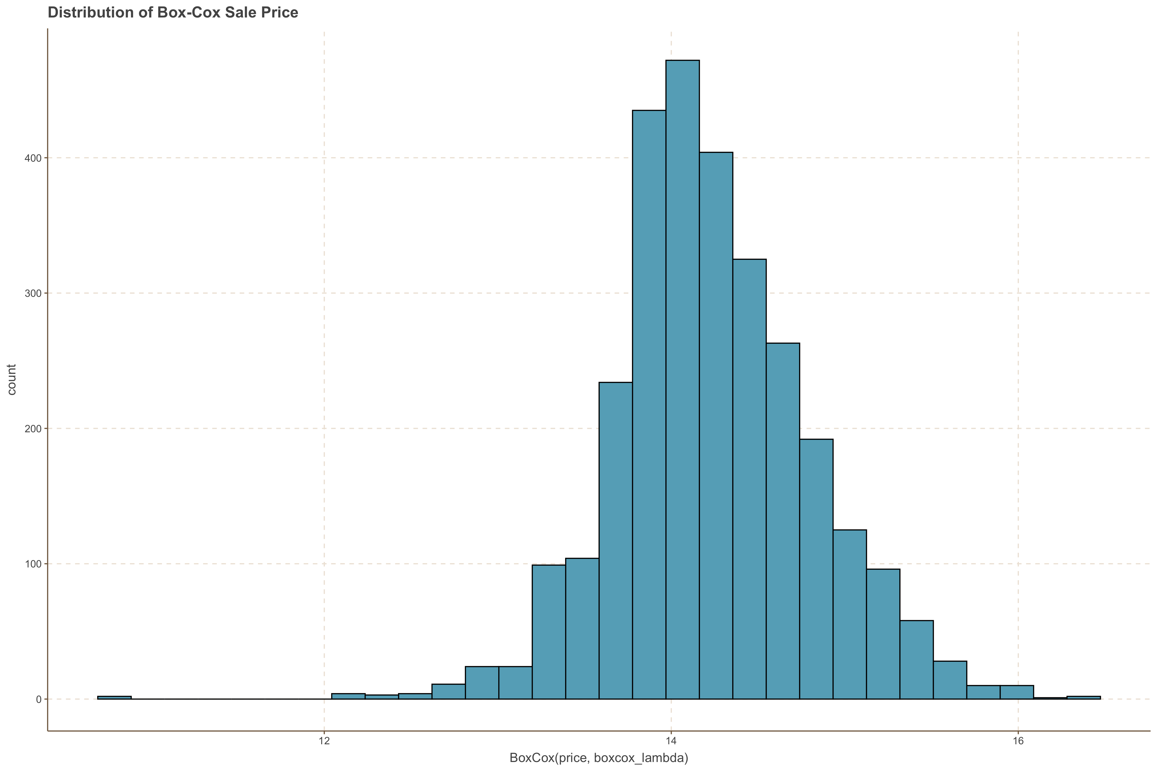
boxcox_lambdaames %>%
ggplot(., aes(x = BoxCox(price, boxcox_lambda))) +
geom_histogram( color = 'black', bins = 30 ) +
ggtitle("Distribution of Box-Cox Sale Price")