Classification with k-Nearest Neighbors
K-Nearest Neighbors is perhaps the most intuitive of the learning techiniques in Machine Learning. In many ways, the approach mirrors how we intuitively estimate or assess the value of products and services. We often look at comparable items to determine the value of a product or service of interest.
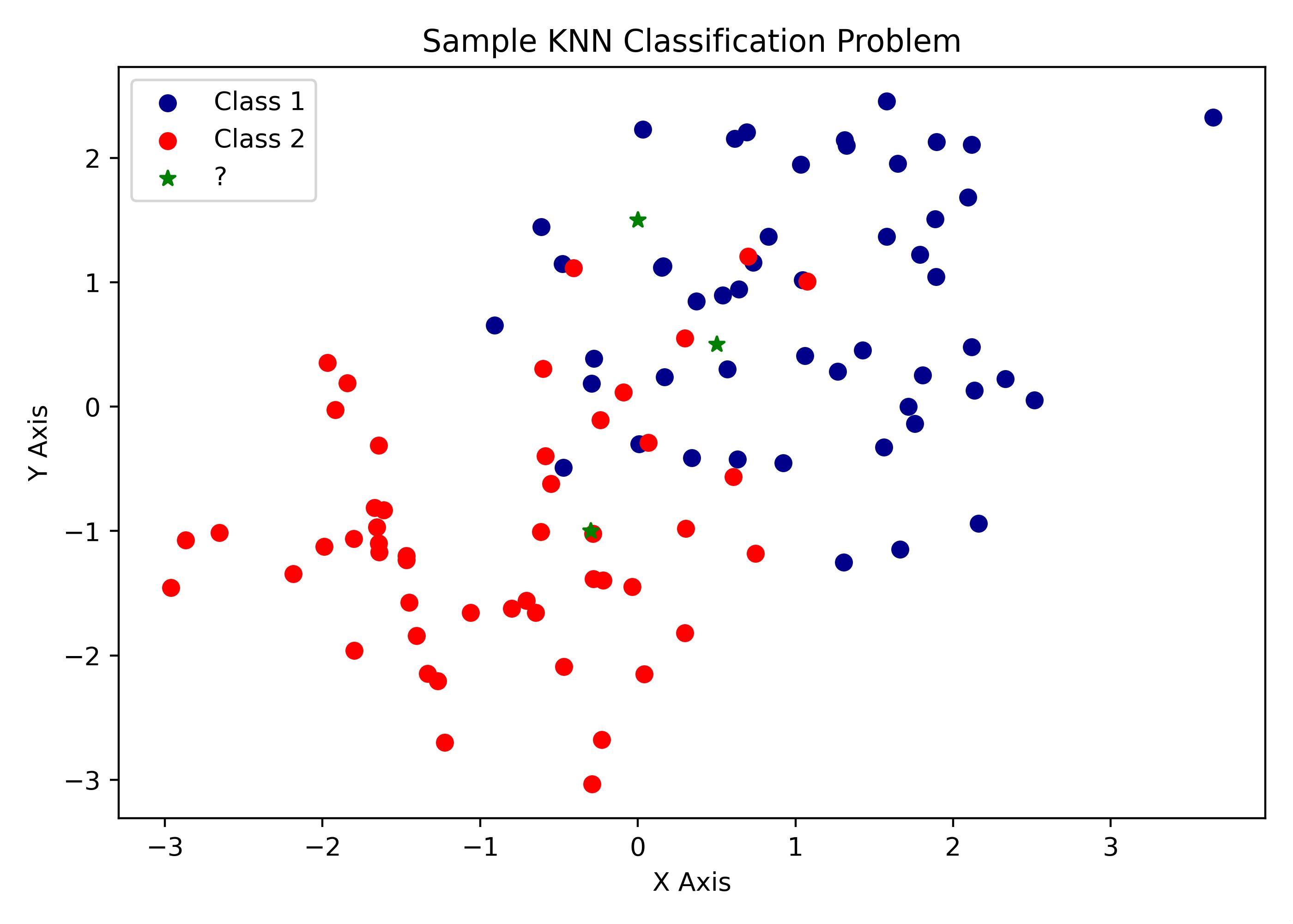
The K-Nearest Neighbors classification algorithm works in the same way. It uses vector based distances to determine the closest $K$ neighbors and takes the majority class of the neighbors as the new class designation of the target observation. The visualization below illustrates the problem statement and why KNN can be an effective solution.
What is KNN?
K-Nearest Neighbors (KNN) is a non-parametric method that predicts the outcome for an input based on the k most similar observations. It is described as non-parametric because it does not involve calculating parameters as linear regression does. This characteristic offers several advantages, such as eliminating the need to assume a specific distribution of the data. Its simplicity facilitates understanding and implementation, and it performs exceptionally well in capturing complex relationships, especially as the value of k increases. KNN can be adapted for both classification and regression tasks with minimal modifications.
At the heart of the KNN method is the principle that observations with similar features are likely to yield similar target variables. Therefore, to predict the class or target variable of a query input, we simply need to identify the most similar observations. But how do we determine which observations are similar to the input?
Distance Metrics
Various classes of distance metrics exist to measure the similarity between observations, with a particular focus on two of the most prevalent geometric distances: Euclidean Distance and Cosine Similarity.
1. Euclidean Distance
Euclidean distance is the most widely used geometric distance metric, measuring the straight-line distance between two points in a vector space. Mathematically, it is defined as:
$$d(x, y) = \sqrt{\sum_{i=1}^{n} (x_i - y_i)^2}$$
where $x$ and $y$ are vectors.
In a 2-D vector space, the formula expands to:
$$d(x, y) = \sqrt{(x_1 - x_2)^2 + (y_1 - y_2)^2}$$
For instance, consider two points $A = (6.3, 4.1)$ and $B = (3.2, 1.7)$. The Euclidean distance between these points is calculated as follows:
$$d(A, B) = \sqrt{(6.3 - 3.2)^2 + (4.1 - 1.7)^2} = \sqrt{9.61 + 5.76} = \sqrt{15.37} \approx 3.92$$
Implementation in Python
import numpy as np

a = np.array([6.3, 4.1])
b = np.array([3.2, 1.7])

d = np.sqrt( np.sum( (a - b)**2 ) )
d2. Cosine Similarity
The cosine similarity is the measure of similarity between two vectors. More precisely, it is the cosine measure of the angle between two vectors.
Mathematically, it is represented as:
$$ d(a,b) = \frac{ a*b } { |a| |b| } $$
where:
$a*b$ is the dot product of vectors
$ |a|$ and $|b|$ are the dot products of the vectors
The formular can be expanded on with summation definitions as follows:
$$ d(a, b) = \frac { \sum_{i=1}^n {a_i b_i} } { \sqrt { \sum_{i=1}^n {a_i^2}} \sqrt {\sum_{i=1}^n{b_i^2}} } $$
For example:
$$ d(a, b) = \frac { (6.3*3.2) + (4.1*1.7) } { \sqrt { (6.3^2) + (4.1^2)} \sqrt { (3.2^2) + (1.7^2) } } $$ $$ d(a, b) = \frac {27.13} { 7.516 * 3.623} $$ $$ d(a, b) = \frac {27.13} {27.2368} $$ $$ d(a, b) = .996 $$
np.dot(a, b)/(np.sqrt(np.dot(a, a)) * np.sqrt( np.dot(b, b) ))The K Nearest Neighbor Algorithm
Let's delve into implementing the K-Nearest Neighbors (KNN) algorithm. Below, I'll outline the process using pseudo-code, bearing in mind that this implementation is object-oriented. The approach might vary slightly in a functional programming context.
Initialization
Euclidean Distance Calculation
Core Algorithm
Result
Implementation in Python
Below is a sample object oriented implementation of the KNN Algorithm in Python.
class KNearestNeighborClassifier:

    """ Implements the KNN Classifier Algorithm using Euclidean Distance """

    def __init__(self, features, labels, input_x, k_neighbors=3):
        # feature datasets
        self.features = features
        self.labels = labels

        # values to be classified
        self.input_x = input_x

        # Number of observations
        self.n_obs = features.shape[1]

        # set number of neighbors
        self.k_neighbors = k_neighbors
        self.nearest_neighbors = {}


    def euclidean_distance(self, arr_x, arr_y):
        """ Computes the Euclidean Distance """
        return np.sqrt( np.sum( (arr_x - arr_y) ** 2 ) )


    def k_nearest_neighbor(self):
        for obs in range(self.n_obs):
            distance = self.euclidean_distance(self.input_x, self.features[:, obs])

            if len(self.nearest_neighbors) >= self.k_neighbors:
                self.nearest_neighbors = {k:v for k,v in sorted( self.nearest_neighbors.items(), key=lambda x:x[1]) }
                if distance < list(self.nearest_neighbors.values())[-1]:
                    self.nearest_neighbors.popitem()
                    self.nearest_neighbors[obs] = distance

            else:
                self.nearest_neighbors[obs] = distance

        return self.nearest_neighbors


    def predict_class(self):
        # compute nearest neighbors
        self.k_nearest_neighbor()

        # retrieve predicted class based on votes/max counts of class of the neighbors
        predicted_labels = [ self.labels[index] for index in self.nearest_neighbors.keys()]
        majority_class = { label: predicted_labels.count(label) for label in set(predicted_labels) }
        for k, v in majority_class.items():
            if v == max(majority_class.values()):
                return f"Majority Class: {k},  Class Votes: {majority_class}"
Testing the Algorithm on Sample Data
With the KNN class completed, I will test the implementation of the algorithm on some same data.
import pandas as pd

dataset = pd.read_csv('sample.txt')
dataset.head()| X | Y | class | |
|---|---|---|---|
| 0 | 1.206922 | 2.206818 | A |
| 1 | 3.235168 | 1.338481 | A |
| 2 | 1.778673 | 1.464483 | A |
| 3 | -0.725584 | 1.234910 | A |
| 4 | 0.329946 | 0.033291 | A |
Visualizing the dataset
A visualization step will best illustrustate the datasets and the observation for which we are attempting to make predictions.
import matplotlib.pyplot as plt

%matplotlib inline
%config InlineBackend.figure_format = 'retina'

fig = plt.figure(figsize=(7,5), dpi=250)
plt.scatter(dataset[dataset['class']=='A' ]['X'], dataset[dataset['class'] == 'A']['Y'], label='Class A ')
plt.scatter(dataset[dataset['class']=='B' ]['X'], dataset[dataset['class'] == 'B']['Y'], label='Class B ')


plt.scatter( np.array([0.5, -0.3, 0,]), np.array([0.5, -1, 1.5]), label='?', marker='h', linewidths=3, color='seagreen')
plt.annotate('x', (0.5, 0.5 ), fontsize=8, ha='center' )
plt.annotate('y', (-0.3, -1), fontsize=8, ha='center' )
plt.annotate('z', (0, 1.5), fontsize=8, ha='center' )


plt.legend(loc='upper left')
plt.title('Distribution of Class A & B')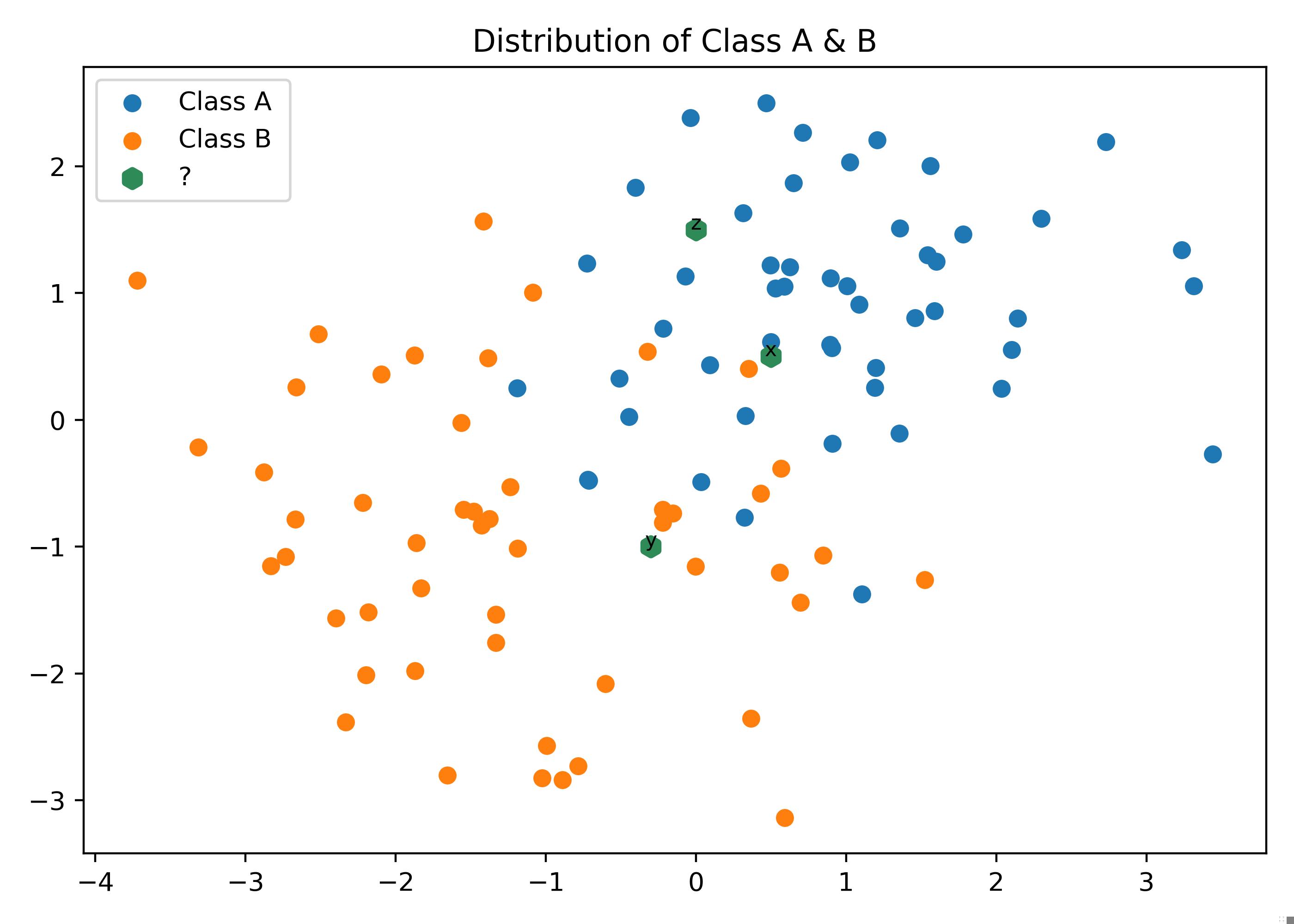
Executing kNN Classifier
To run the kNN algorithm, initialize the three unknown data points as
# new points
x_inputs = np.array([ [0.5, 0.5], [-0.3, -1], [0, 1.5] ])

features = np.array([ dataset.X, dataset.Y  ])
labels = dataset['class']
Generating Predictions
The code below initializes the
# Iterating through the new points for classification
for x_input in x_inputs:
    print(x_input)
    knn_model = KNearestNeighborClassifier( features=features, labels=labels, input_x=x_input, k_neighbors=3)
    neighbors = knn_model.k_nearest_neighbor()
    print("The nearest neighbors are: ", neighbors)
    print(knn_model.predict_class(), '\n')