Bilateral Filter
The bilateral filter builds on top of the Gaussian filter by adding an intensity parameter in estimating the weights of the kernel. Recall, the Gaussian filter is spatial in nature, with weights of the kernel decreasing with increase in distance from the center pixel. While this is useful for noise reduction, it can lead to loss of edges in an image (also known as boundaries).
For example, imagine that the center pixel is of value 255 (white) and the neighborhood pixel, 4 closest in this case, are split between 2 255(white) pixels and 0(black) pixels. The Gaussian filter will assign similar weights to the kernel points corresponding to the pixels, thereby making their influence equal. This will result in loosing edges and boundaries.
To mitigate this, the bilateral filter adds a tonal intensity parameter which assigns higher weight to the kernel when the pixel intensity is closer to the intensity of the center image and vice versa. This allows for the preservation of boundaries in the image.
OpenCV2 provides a utility method to run the bilateral filter. The method is bilateralFilter() and it takes the following arguments:
- $src$: source image
- $ksize$: size of the kernel
- $sigmaSpace$: Spatial parameter
- $sigmaColor$: Tonal intensity parameter
- $borderType$: Border type
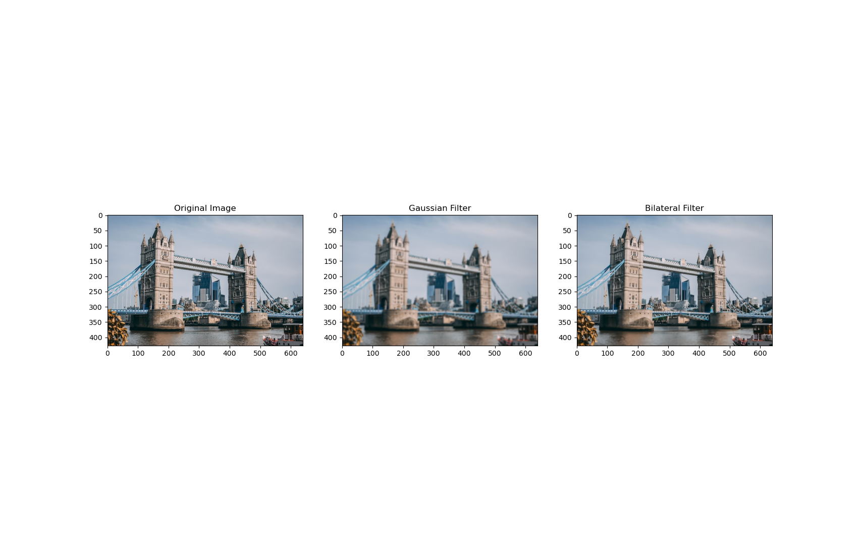
In the example, below we demonstrate the bilateral filter and compare it to the Gaussian Filter.
import cv2
import numpy as np
import matplotlib.pyplot as plt

%matplotlib inline
%config InlineBackend.figure_format = 'retina'
img = cv2.imread('tower_bridge.jpg')
img = cv2.cvtColor(img, cv2.COLOR_BGR2RGB)
# plot the image
plt.imshow(img)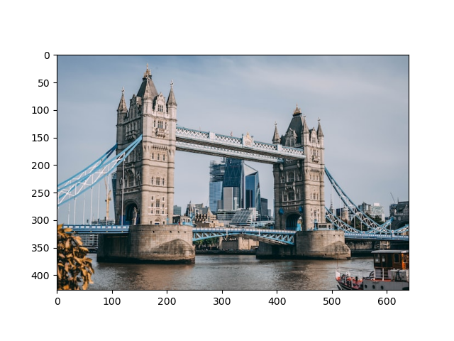
Now we run both Gaussian Filter and Bilateral filter for comparison.
gaussian_filter = cv2.GaussianBlur(img, (7,7), 2)
bilateral_filter = cv2.bilateralFilter(img, 7, sigmaSpace=50, sigmaColor=90, borderType=cv2.BORDER_CONSTANT)
fig = plt.figure(figsize=(17, 11))
fig.add_subplot(131)
plt.imshow(img)
plt.title('Original Image')
fig.add_subplot(132)
plt.imshow(gaussian_filter)
plt.title('Gaussian Filter')
fig.add_subplot(133)
plt.imshow(bilateral_filter)
plt.title('Bilateral Filter')