Gaussian Filter

The Gaussian filter, also know as the Gaussian blur is a commonly used spatial filter for noise reduction. The difference of this filter against the average filter is that, the kernel weights are approximated from the Gaussian distribution and have spatial in nature. That is spatial weighting assign weights to the kernel based on distance from the center pixel. More concretely, the center kernel weight is higher in magnitude to the neighbors and the neighbors weight decrease as kernel coordinate are further from the center.

Below is an example of an approximated Gaussian kernel.

$$ k = \frac {1}{16} \begin{pmatrix} 1 & 2 & 1 \\ 2 & 4 & 2 \\ 1 & 2 & 1 \end{pmatrix} $$

OpenCV provides yet another convenient method to implement Gaussian Filters. The method is cv2.GaussianBlur() and it takes the following arguments:

1. $src$: source image
2. $ksize$: size of kernel in tuple i.e. (3, 3)
3. $radius$: sigma value for the distribution

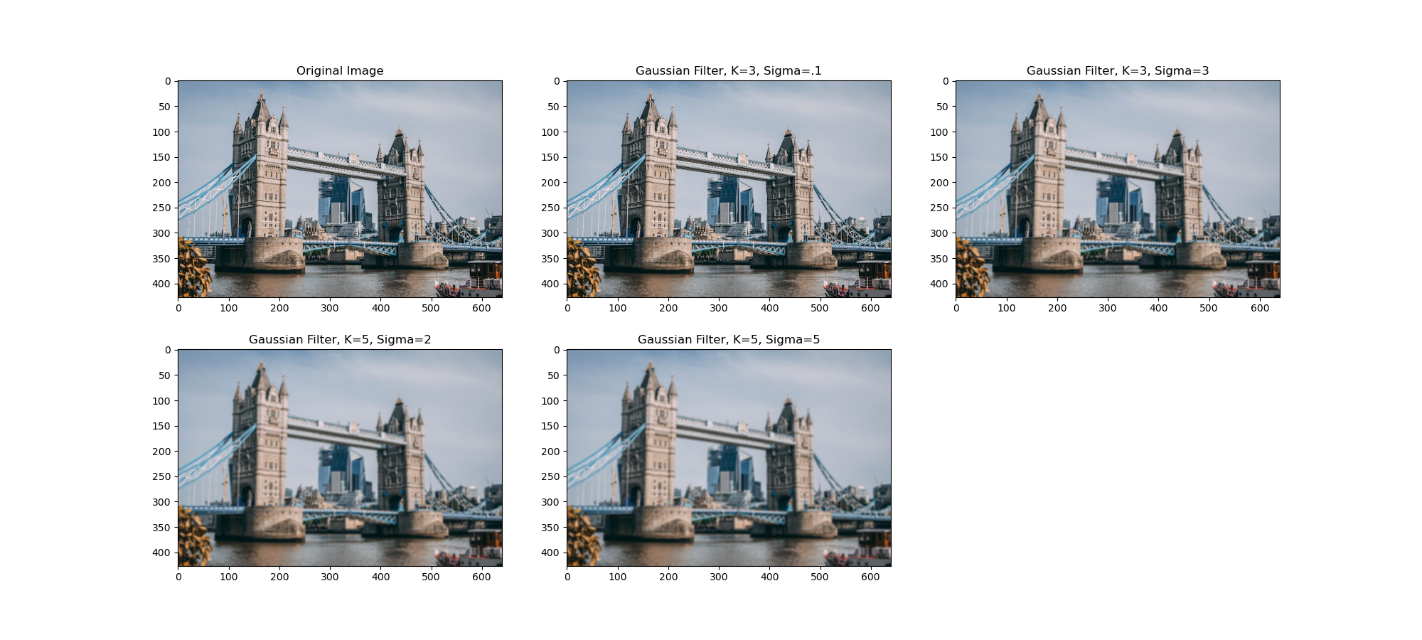
In the example below, we implement the GaussianBlur() with a few varying dimensions:

1. $k=3, \sigma=.1$, $k=3, \sigma=3$, $k=5, \sigma=2$, $k=5, \sigma=5$

import cv2
import numpy as np
import matplotlib.pyplot as plt

%matplotlib inline
%config InlineBackend.figure_format = 'retina'

img = cv2.imread('tower_bridge.jpg')
img = cv2.cvtColor(img, cv2.COLOR_BGR2RGB)
    
# plot the image
plt.imshow(img)

Implementing the filter on img

gauss_k3_1 = cv2.GaussianBlur(img, (3,3), .1)
gauss_k3_3 = cv2.GaussianBlur(img, (3,3), 3)
gauss_k5_1 = cv2.GaussianBlur(img, (5,5), 2)
gauss_k5_5 = cv2.GaussianBlur(img, (5,5), 5)

fig = plt.figure(figsize=(20, 9))

fig.add_subplot(231)
plt.imshow(img)
plt.title('Original Image')

fig.add_subplot(232)
plt.imshow(gauss_k3_1)
plt.title('Gaussian Filter, K=3, Sigma=.1')

fig.add_subplot(233)
plt.imshow(gauss_k3_3)
plt.title('Gaussian Filter, K=3, Sigma=3')


fig.add_subplot(234)
plt.imshow(gauss_k5_1)
plt.title('Gaussian Filter, K=5, Sigma=2')

fig.add_subplot(235)
plt.imshow(gauss_k5_5)
plt.title('Gaussian Filter, K=5, Sigma=5')