Histogram Gray Scales

A histogram on an image provides useful information about the distribution of tonal intensity of an image. Visually, the histogram tells us the image composition. If the histogram is dense on lower values (closer to 0), then we know the image largely contains darkers colors while if it is dense on higher values, the image largely contains brighter colors.

Reading a sample image

import cv2
import numpy as np
import matplotlib.pyplot as plt

%matplotlib inline
%config InlineBackend.figure_format = 'retina'

img = cv2.imread('natural_history.jpg')
img = cv2.cvtColor(img, cv2.COLOR_BGR2RGB)
    
# image show    
plt.imshow(img)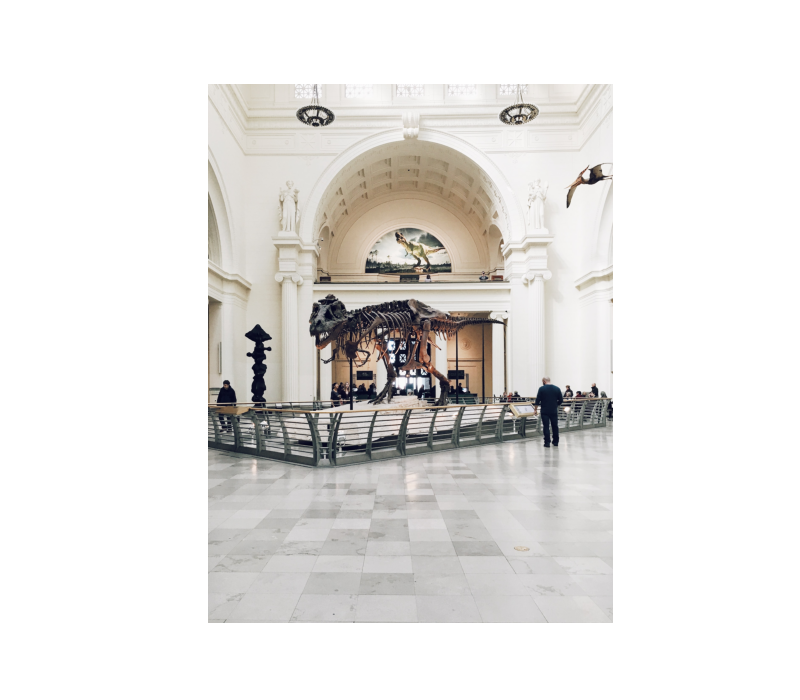

img.shape

(2560, 1920, 3)

Grayscale Conversion

it is very common in Computer to convert the image into GRAYSCALE and perform operations. Its reduces complexity of operations and can always be converted back to color image. In this example, we implement grayscale conversion.

gray_img = cv2.cvtColor(img, cv2.COLOR_BGR2GRAY)

Generating Histogram

The cv2.calcHist() returns an array of pixels equal to the size of the image ranging in intensity from 0 - 255. It takes the following arguments:

1. The input image
2. The channels we wish to computer histogram.
3. Mask, if defined
4. histSize: the number of bins 255 (the x-axis)
5. The range of intensity (0, 256)

histogram = cv2.calcHist([gray_img], [0], None, [256], [0, 256])

# plotting the histogram
plt.figure(figsize=(8, 4))        
plt.plot(histogram)
plt.title('Histogram of Car Image')
plt.xlabel('Pixel Intensity')
plt.ylabel('# of pixels on image')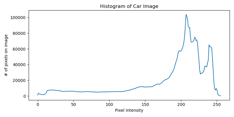

Notice that the distribution is skewed to the left with high density of pixes in the higher pixel values. This suggest the image is mostly white.