Histogram Equalization

Histogram Equalization is the process of normalizing the intensity of the individual pixel against its respective probability (the likelihood of that pixel intensity value in the image). The outcome of this operation is an image is often has higher, perhaps better contrast than the original image

Mathematically, histogram equalization is defined by the following formular

$$ img_{eq} = (levels-1) \sum_{i=1}^{n}{ p_i} $$

where:
$p_i$: probability density values at pixel intensity $i$
$levels$: total intensity levels (i.e. grayscale = 8, (0-7)

Example:

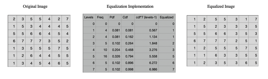
Suppose we have a $7x7$ image with pixels values on the left matrix below. The histogram equalization process follows the following operations:

1. 1. We first establish a gray scale level of pixels and compute frequency from image
2. 2. Compute the pdf against the frequency: $\frac{freq}{total\ pixels}$
3. 3. Compute the cumulative density distribution i.e. cumulative sum of pdfs
4. 4. Multiply cdf by total gray levels - 1 (7)
5. 5. Round the resulting value to get equalized pixel.
6. 6. Finally, map the original gray scale pixel to new equalized pixel

Implementation in OpenCV

import cv2
import numpy as np
import matplotlib.pyplot as plt

%matplotlib inline
%config InlineBackend.figure_format = 'retina'

cat_img = cv2.imread('cat.png')
cat_img = cv2.cvtColor(cat_img, cv2.COLOR_BGR2RGB)
plt.imshow(cat_img)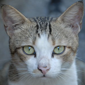

Converting to Grayscale

cat_img_gray = cv2.cvtColor(cat_img, cv2.COLOR_RGB2GRAY)
plt.imshow(cat_img_gray, cmap='gray')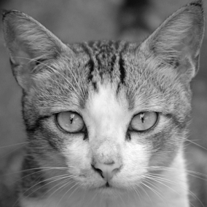

Equalization

cat_img_gray_eq = cv2.equalizeHist(cat_img_gray)

fig = plt.figure(figsize=(15, 10))

fig.add_subplot(131)
plt.imshow(cat_img)
plt.title('Original Image')
plt.axis('off')

fig.add_subplot(132)
plt.imshow(cat_img_gray, cmap='gray')
plt.title('Grayscale Image')
plt.axis('off')

fig.add_subplot(133)
plt.imshow(cat_img_gray_eq, cmap='gray')
plt.title('Histogram Equalized Image')
plt.axis('off')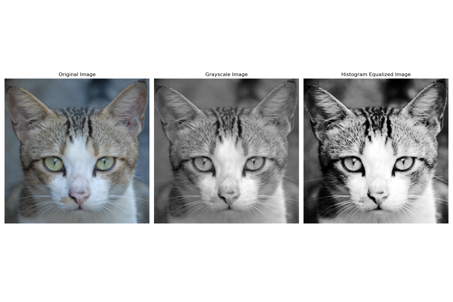

Notice that the equalized histogram image has better contrast than the original and gray scale images.