Kernel Convolutions with OpenCV
Convolution with OpenCV work in much the same way as the convolution with ndimage. We will use an example of a butterfly image and apply the following kernels.
$$ kernel_1= \begin{pmatrix} 1 & 1 & 1 \\ 1 & 1 & 1 \\ 1 & 1 & 1 \end{pmatrix}, kernel_2 = 1/9 * \begin{pmatrix} 1 & 1 & 1 \\ 1 & 1 & 1 \\ 1 & 1 & 1 \end{pmatrix}, kernel_3 = \begin{pmatrix} -1 & -1 & -1 \\ -1 & 8 & -1 \\ -1 & -1 & -1 \end{pmatrix}$$
Implementation in OpenCV
import cv2
import numpy as np
import matplotlib.pyplot as plt

%matplotlib inline
%config InlineBackend.figure_format = 'retina'
img = cv2.imread('butterfly.jpg')
img = cv2.cvtColor(img, cv2.COLOR_BGR2RGB)
# image show
plt.imshow(img)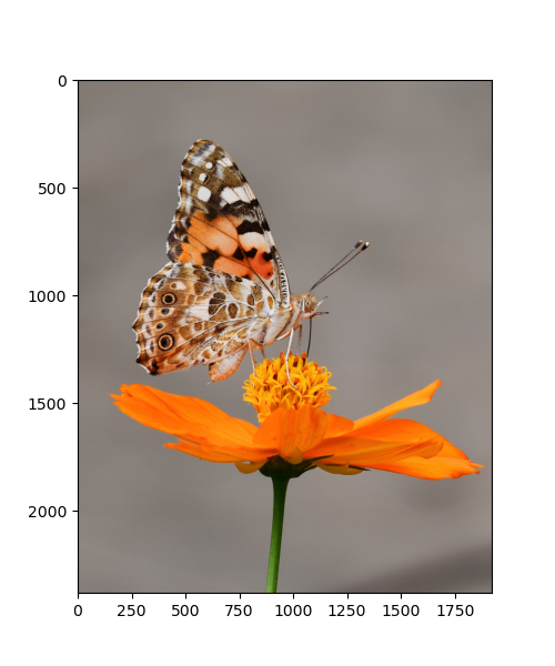
Defining Kernels
kernel_1 = np.ones(shape=(3,3))
kernel_2 = 1/9*(kernel_1)

kernel_3 =  -1*(np.ones(shape=(3,3)))
kernel_3[1,1] = 8

kernel_1, kernel_2, kernel_3
(array([[1., 1., 1.],
[1., 1., 1.],
[1., 1., 1.]]),
array([[0.11111111, 0.11111111, 0.11111111],
[0.11111111, 0.11111111, 0.11111111],
[0.11111111, 0.11111111, 0.11111111]]),
array([[-1., -1., -1.],
[-1., 8., -1.],
[-1., -1., -1.]]))
Convolution Implementation
To implement a convolution with opencv, we use the method cv2.filter2D(). The method takes the following arguments:
- 1. src: input image we wish to convolve
- 2. ddepth: destination depth (). In this case we use -1 to signify the source image depth is to be used for the destination image
- 3. kernel: the kernel matrix
convolved_k1 = cv2.filter2D(img, -1, kernel_1)
convolved_k2 = cv2.filter2D(img, -1, kernel_2)
convolved_k3 = cv2.filter2D(img, -1, kernel_3)
Visualizing the convolution outcome
fig = plt.figure(figsize=(8,10))

fig.add_subplot(221)
plt.imshow(img)
plt.title('Original Image')

fig.add_subplot(222)
plt.imshow(convolved_k1)
plt.title('Convolution K1')

fig.add_subplot(223)
plt.imshow(convolved_k2)
plt.title('Convolution K2')


fig.add_subplot(224)
plt.imshow(convolved_k3)
plt.title('Convolution K3')

plt.tight_layout()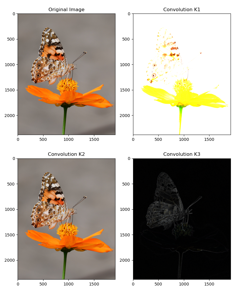
Notice that a couple of useful things:
- 1. The first kernel simply resulted in the sum of neighbor pixels to the center pixel. This has the effect of brightening the image overall.
- 2. The second kernel is takes the weighted sum of the neighbor pixels and averages them. This often has the effect of bluring the image.
- 3. The third kernel which is often used for enhancing edges magnifies the center pixel with a high weight while reducing the neighboring pixels with a negative weight.